2019年6月 – TauStation

微分の定義

初等的な微分の定義は以下の通り。

(1) $\begin{equation*} f'(x) = \frac{d f(x)}{dx} = \lim_{\Delta x \rightarrow 0} \frac{f(x + \Delta x) - f(x)}{\Delta x} \end{equation*}$

関数の積・商の微分

関数の積の微分

(2) $\begin{equation*} f(x) = u(x) v(x) \rightarrow f'(x) = u(x) v'(x) + u'(x) v(x) \end{equation*}$

(3) $\begin{equation*} f'(x) = \lim_{\Delta x \rightarrow 0} \frac{u(x + \Delta x) v(x + \Delta x) - u(x) v(x)}{\Delta x} \end{equation*}$

ここで

(4) $\begin{eqnarray*} u(x + \Delta x) &=& u(x) + u'(x) \Delta x + o({\Delta x}^2) \\ v(x + \Delta x) &=& v(x) + v'(x) \Delta x + o({\Delta x}^2) \end{eqnarray*}$

したがって、

(5) $\begin{equation*} u(x + \Delta x) v(x + \Delta x) = u(x) v(x) + u(x) v'(x) \Delta x + u'(x) v(x) \Delta x + o({\Delta x}^2) \end{equation*}$

これより以下を得る。

(6) $\begin{eqnarray*} f'(x) &=& \lim_{\Delta x \rightarrow 0} \frac{u(x) v'(x) \Delta x + u'(x) v(x) \Delta x + o({\Delta x}^2)}{\Delta x} \\ &=& u(x) v'(x) + u'(x) v(x) \end{eqnarray*}$

関数の商の微分

(7) $\begin{equation*} f(x) = \frac{v(x)}{u(x)} \rightarrow f'(x) = \frac{u(x) v'(x) - u'(x) v(x)}{u(x) ^2} \end{equation*}$

(8) $\begin{equation*} f(x) = \frac{v(x)}{u(x)} \Leftrightarrow v(x) = f(x) u(x) \end{equation*}$

(9) $\begin{equation*} v'(x) = f'(x) u(x) + f(x) u'(x) = f'(x) u(x) + \frac{v(x) u'(x)}{u(x)} \end{equation*}$

これより(7)を得る。

合成関数の微分

(10) $\begin{eqnarray*} y = f(u(x)) & \rightarrow & \frac{dy}{dx} = f'(u(x))u'(x) \\ &{\rm or}& \\ \frac{dy}{dx} &=& \frac{dy}{du} \frac{du}{dx} \end{eqnarray*}$

$u(x + \Delta x) - u(x) = \Delta u(x)$ とおくと、

(11) $\begin{eqnarray*} && lim_{x \rightarrow \infty} \frac{f(u(x + \Delta x)) - f(u(x))}{\Delta x} \\ &=& lim_{x \rightarrow \infty} \frac{f(\Delta u(x)) - f(u(x))}{\Delta u(x)} \frac{\Delta u(x)}{\Delta x} \\ &=& f'(u(x))u'(x) \end{eqnarray*}$

逆関数の微分

(12) $\begin{eqnarray*} y = f^{-1}(x) & \rightarrow & \frac{dy}{dx} = \frac{1}{f'(x)} \\ &{\rm or}& \\ \frac{dx}{dy} &=& \frac{1}{\frac{dy}{dx}} \end{eqnarray*}$

(13) $\begin{equation*} y = f^{-1}(x) \rightarrow f(y) = x \end{equation*}$

とおいて、合成関数の微分より、

(14) $\begin{eqnarray*} f'(y) \frac{dy}{dx} = 1 \\ \therefore \frac{dy}{dx} = \frac{1}{f'(y)} \end{eqnarray*}$

媒介変数表示

(15) $\begin{equation*} x = u(t), y = v(t) \rightarrow \frac{dy}{dx} = \frac{\frac{dy}{dt}}{\frac{dx}{dt}} = \frac{v'(t)}{u'(t)} \end{equation*}$

$\Delta u(t) = u(t + \Delta t) - u(t)$ 、 $\Delta v(t) = v(t + \Delta t) - v(t)$ とおいて、

(16) $\begin{equation*} \lim_{n \rightarrow \infty} \frac{\Delta v(t)}{\Delta u(t)} = \lim_{n \rightarrow \infty} \frac{v(t + \Delta t) - v(t)}{\Delta t} \frac{\Delta t}{u(t + \Delta t) - u(t)} = \frac{v'(t)}{u'(t)} \end{equation*}$

概要

中心極限定理(central limit theorem: CLT)は、一言で言えば次のようになる。「母集団がどのような確率分布に従うとしても、標本の数を十分大きくしたときには、その合計値あるいは標本平均は、正規分布に従う」

具体的には、母集団の平均を $\mu$ 、標準偏差を $\sigma$ とし、 $n$ が十分に大きいとき、

標本の合計 $S_n = \sum X_{i}$ は正規分布 $N(n \mu,n\sigma^2)$ に従う

標本平均 $\overline{X}_n = \frac{1}{n} \sum X_{i}$ は正規分布 $N(\mu, \frac{\sigma^2}{n})$ に従う

実用

たとえば、サイコロを $n$ 回振った目の合計を考える。全て1（合計が $n$ ）や全て6（合計が6 $n$ ）というケースは稀なので、その間の値になりそうだと予想される。

中心極限定理を用いると、 $n$ 個のサイコロの目の平均と分散より、 $n$ 個のサイコロの目の合計は、 $N( \frac{7}{2} , \frac{35}{12n})$ に従うことになる。

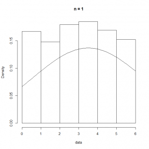
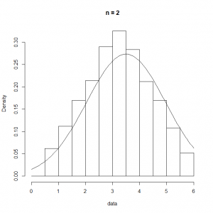
これをRの下記コードで試してみた。一回の試行でサイコロを投げる回数をn.dicesに設定して、その平均を求める試行を1000回繰り返す。

n.dices <- 5
n.data <- 1000
num.data <- lambda * t.obs

data <- c()
for (i in 1:n.data) {
  data <- c(data, mean(as.integer(runif(n.dices, min=1, max=7))))
}

ranks <- seq(0, 6, 0.5)
hist(data, breaks=ranks, prob=T, main=paste("n =", n.dices))
curve(dnorm(x, 7/2, 35/12/n.dices), add=TRUE)

n.dices <- 5

n.data <- 1000

num.data <- lambda * t.obs

data <- c()

for (i in 1:n.data) {

data <- c(data, mean(as.integer(runif(n.dices, min=1, max=7))))

}

ranks <- seq(0, 6, 0.5)

hist(data, breaks=ranks, prob=T, main=paste("n =", n.dices))

curve(dnorm(x, 7/2, 35/12/n.dices), add=TRUE)

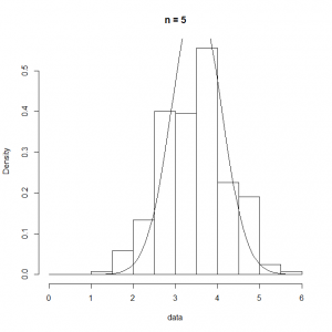
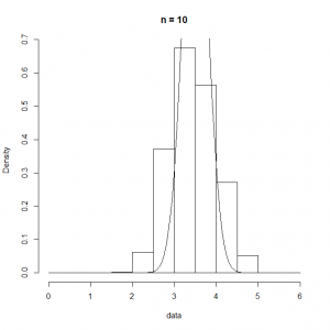
n.dicesの回数を変化させた実行結果は以下の通りで、このケースの場合は、 $n$ =10程度でもかなり平均の周りに尖った分布となる。

TauStation

月別: 2019年6月

微分の公式