DecisionTreeClassifier – Treeオブジェクト・再帰表示など

2020-05-31 / tau / コメントする

概要

Scikit-learnの決定木モデル、DecisionTreeClassifierについていろいろ試した際のコードをストック。

Treeオブジェクト内容確認

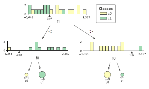
DecisionTreeClassifierオブジェクトのプロパティーtree_はデータセットに対して生成された決定木の構造が保存されている。以下はその内容を確認するためのコード。

import numpy as np
import matplotlib.pyplot as plt
from sklearn.datasets import make_moons
from sklearn.tree import DecisionTreeClassifier

X, y = make_moons(n_samples=20, noise=0.25, random_state=3)

treeclf = DecisionTreeClassifier(random_state=0)
treeclf.fit(X, y)

tree = treeclf.tree_

n_nodes = tree.node_count
children_left = tree.children_left
children_right = tree.children_right
features = tree.feature
thresholds = tree.threshold
value = tree.value

print("number of nodes: {}".format(n_nodes))
print("Chlidren(Left) : {}".format(children_left))
print("Chlidren(Right): {}".format(children_right))
print("Features       : {}".format(features))
print("Thresholds     : {}".format(np.round(thresholds, 3)))
print("Values:\n{}".format(value))

print()

for i in range(n_nodes):
    print("Node-{}".format(i), end="")
    print("(Feature[{:2d}]<{:6.3f}):"\
        .format(features[i], thresholds[i]), end="")
    print("LeftNode[{:2d}], RightNode[{:2d}]"\
        .format(children_left[i], children_right[i]))

import numpy as np

import matplotlib.pyplot as plt

from sklearn.datasets import make_moons

from sklearn.tree import DecisionTreeClassifier

X, y = make_moons(n_samples=20, noise=0.25, random_state=3)

treeclf = DecisionTreeClassifier(random_state=0)

treeclf.fit(X, y)

tree = treeclf.tree_

n_nodes = tree.node_count

children_left = tree.children_left

children_right = tree.children_right

features = tree.feature

thresholds = tree.threshold

value = tree.value

print("number of nodes: {}".format(n_nodes))

print("Chlidren(Left) : {}".format(children_left))

print("Chlidren(Right): {}".format(children_right))

print("Features : {}".format(features))

print("Thresholds : {}".format(np.round(thresholds, 3)))

print("Values:\n{}".format(value))

print()

for i in range(n_nodes):

print("Node-{}".format(i), end="")

print("(Feature[{:2d}]<{:6.3f}):"\

.format(features[i], thresholds[i]), end="")

print("LeftNode[{:2d}], RightNode[{:2d}]"\

.format(children_left[i], children_right[i]))

Treeクラスはツリー内の各ノードの情報を1次元の配列でもっていて、子ノードを参照するにはノード番号に対応する配列のインデックスを参照する。Treeクラスが持っている主なプロパティーは以下の通り。

node_count: ツリーが持つ全ノード数。
children_left, children_right: 各ノードの左／右の子ノードの番号を格納した1次元配列。
feature: 各ノードを分割する際に使われる特徴量の番号を格納した1次元配列。
threshold: 各ノードをfeatureで示された特性量で分割する際の閾値を格納した1次元配列。
value: 各ノードにおける、各クラスのデータ数。クラス数分のデータを格納した1次元配列1つだけを要素とする2次元配列を、ノード数分だけ集めた3次元配列。

コードの実行結果は以下の通り。

number of nodes: 7
Chlidren(Left) : [ 1  2 -1 -1  5 -1 -1]
Chlidren(Right): [ 4  3 -1 -1  6 -1 -1]
Features       : [ 1  0 -2 -2  0 -2 -2]
Thresholds     : [ 0.072 -0.643 -2.    -2.     1.536 -2.    -2.   ]
Values:
[[[10. 10.]]

 [[ 1.  9.]]

 [[ 1.  0.]]

 [[ 0.  9.]]

 [[ 9.  1.]]

 [[ 9.  0.]]

 [[ 0.  1.]]]

Node-0(Feature[ 1]< 0.072):LeftNode[ 1], RightNode[ 4]
Node-1(Feature[ 0]<-0.643):LeftNode[ 2], RightNode[ 3]
Node-2(Feature[-2]<-2.000):LeftNode[-1], RightNode[-1]
Node-3(Feature[-2]<-2.000):LeftNode[-1], RightNode[-1]
Node-4(Feature[ 0]< 1.536):LeftNode[ 5], RightNode[ 6]
Node-5(Feature[-2]<-2.000):LeftNode[-1], RightNode[-1]
Node-6(Feature[-2]<-2.000):LeftNode[-1], RightNode[-1]

number of nodes: 7

Chlidren(Left) : [ 1 2 -1 -1 5 -1 -1]

Chlidren(Right): [ 4 3 -1 -1 6 -1 -1]

Features : [ 1 0 -2 -2 0 -2 -2]

Thresholds : [ 0.072 -0.643 -2. -2. 1.536 -2. -2. ]

Values:

[[[10. 10.]]

[[ 1. 9.]]

[[ 1. 0.]]

[[ 0. 9.]]

[[ 9. 1.]]

[[ 9. 0.]]

[[ 0. 1.]]]

Node-0(Feature[ 1]< 0.072):LeftNode[ 1], RightNode[ 4]

Node-1(Feature[ 0]<-0.643):LeftNode[ 2], RightNode[ 3]

Node-2(Feature[-2]<-2.000):LeftNode[-1], RightNode[-1]

Node-3(Feature[-2]<-2.000):LeftNode[-1], RightNode[-1]

Node-4(Feature[ 0]< 1.536):LeftNode[ 5], RightNode[ 6]

Node-5(Feature[-2]<-2.000):LeftNode[-1], RightNode[-1]

Node-6(Feature[-2]<-2.000):LeftNode[-1], RightNode[-1]

親ノードと子ノードの関係は、たとえばノード0の左右の子ノードはchildren_leftとchildren_rightの0番目の要素からノード1とノード4、ノード1の左右の子ノードはノード2とノード3、という風に追っていくことができる。

valueがややこしい。この配列は各ノードにおけるクラスごとのデータ数を格納している。全体配列の中にこのケースだとノード数に対応する7個の配列が要素として格納されているが、その配列が2次元配列になっていて、その要素の配列がクラスごとのデータを格納した配列になっている。例えば3番目の要素のクラス1の要素を取り出す場合にはvalue[3, 0, 1]と言う風に指定することになる。

Treeのコンソール表示

Treeオブジェクトのツリー構造を確認し、決定境界の描画などの準備とするために書いたコード。決定木の構造をコンソールに表示させる。2つの再帰関数を定義していて、本体は決定木学習後にそれらの関数を呼び出すのみ。

from sklearn.datasets import make_moons
from sklearn.tree import DecisionTreeClassifier

def print_node1(tree, i_node, n_level=0):
    print("{}{:2d}-feature:{:2d}"\
        .format("             " * n_level, i_node, tree.feature[i_node]))
    if tree.children_left[i_node] == -1:
        return
    print_node1(
        tree=tree, i_node=tree.children_left[i_node], n_level=n_level+1)
    print_node1(
        tree=tree, i_node=tree.children_right[i_node], n_level=n_level+1)

def print_node2(tree, i_node, n_level=0):
    if tree.children_left[i_node] == -1:
        print("{}{:2d}-feature:{:2d}"\
            .format("             " * n_level, i_node, tree.feature[i_node]))
        return
    print_node2(
        tree=tree, i_node=tree.children_left[i_node], n_level=n_level+1)
    print("{}{:2d}-feature:{:2d}"\
        .format("             " * n_level, i_node, tree.feature[i_node]))
    print_node2(
        tree=tree, i_node=tree.children_right[i_node], n_level=n_level+1)

X, y = make_moons(n_samples=20, noise=0.25, random_state=3)

treeclf = DecisionTreeClassifier(random_state=0)
treeclf.fit(X, y)

tree = treeclf.tree_

print_node1(tree=tree, i_node=0)
print("-"*40)
print_node2(tree=tree, i_node=0)

from sklearn.datasets import make_moons

from sklearn.tree import DecisionTreeClassifier

def print_node1(tree, i_node, n_level=0):

print("{}{:2d}-feature:{:2d}"\

.format(" " * n_level, i_node, tree.feature[i_node]))

if tree.children_left[i_node] == -1:

return

print_node1(

tree=tree, i_node=tree.children_left[i_node], n_level=n_level+1)

print_node1(

tree=tree, i_node=tree.children_right[i_node], n_level=n_level+1)

def print_node2(tree, i_node, n_level=0):

if tree.children_left[i_node] == -1:

print("{}{:2d}-feature:{:2d}"\

.format(" " * n_level, i_node, tree.feature[i_node]))

return

print_node2(

tree=tree, i_node=tree.children_left[i_node], n_level=n_level+1)

print("{}{:2d}-feature:{:2d}"\

.format(" " * n_level, i_node, tree.feature[i_node]))

print_node2(

tree=tree, i_node=tree.children_right[i_node], n_level=n_level+1)

X, y = make_moons(n_samples=20, noise=0.25, random_state=3)

treeclf = DecisionTreeClassifier(random_state=0)

treeclf.fit(X, y)

tree = treeclf.tree_

print_node1(tree=tree, i_node=0)

print("-"*40)

print_node2(tree=tree, i_node=0)

関数print_node1()は、ツリー構造をルートノードから階層が下がるごとに段下げして表示していく。このため、まず親ノードを表示してから左右の子ノードを引数として再帰呼び出しをしている。

終了条件はノードが子ノードを持たない葉(leaf)であることを利用するが、リーフの時のパラメータは以下の通りで、ここでは左子ノードの番号が−1となることを利用している。

子ノードの番号が−1
特性量の番号が−2
特性量の閾値が−2.0

関数print_node2は、決定木の構造を枝分かれした木の形で表示する。左側のノードから右側に移るのを、コンソール上で上から下に表示していく。手順としては、

リーフノードならノードの内容を出力してリターン
リーフノードでなければ、
1. 左子ノードの処理を呼び出す
2. それが戻ってきたら（左側の全子孫ノードが出力されたら）自身の内容を出力
3. 右子ノードの処理を呼び出す
4. それが戻ってきたら（右側の全子孫ノードが出力されたら）リターン

引数に現在のノードの階層を保持する変数があり、その階層に応じた数のスペースでインデントすることで木の構造を表す。

出力は以下の通り。

 0-feature: 1
              1-feature: 0
                           2-feature:-2
                           3-feature:-2
              4-feature: 0
                           5-feature:-2
                           6-feature:-2
----------------------------------------
                           2-feature:-2
              1-feature: 0
                           3-feature:-2
 0-feature: 1
                           5-feature:-2
              4-feature: 0
                           6-feature:-2

0-feature: 1

1-feature: 0

2-feature:-2

3-feature:-2

4-feature: 0

5-feature:-2

6-feature:-2

----------------------------------------

2-feature:-2

1-feature: 0

3-feature:-2

0-feature: 1

5-feature:-2

4-feature: 0

6-feature:-2

決定木の構築過程の表示

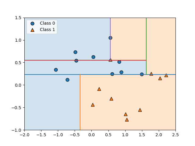
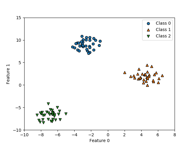
make_monns()による2特性量のデータについて、順次ノードを分割する過程を図で描画するためのコード。

import numpy as np
import matplotlib.pyplot as plt
import matplotlib.patches as patch
from sklearn.datasets import make_moons
from sklearn.tree import DecisionTreeClassifier


def draw_tree_boundary(tree, ax, left, right, bottom, top,
        i_node=0, stop_level=None, n_level=0):

    if tree.children_left[i_node] == -1 or stop_level == n_level:
        fc =\
            'tab:orange' if np.argmax(tree.value[i_node][0])==0 else 'tab:blue'
        rect = patch.Rectangle(xy=(left, bottom),
            width=right-left, height=top-bottom, fc=fc, alpha=0.2)
        ax.add_patch(rect)
        return

    if tree.feature[i_node] == 0:
        f0 = tree.threshold[i_node]
        ax.plot([f0, f0], [top, bottom])
        draw_tree_boundary(tree=tree, ax=ax,
            left=left, right=f0, top=top, bottom=bottom,
            i_node=tree.children_left[i_node],
            stop_level=stop_level, n_level=n_level+1,)
        draw_tree_boundary(tree=tree, ax=ax,
            left=f0, right=right, top=top, bottom=bottom,
            i_node=tree.children_right[i_node],
            stop_level=stop_level, n_level=n_level+1)
    else:
        f1 = tree.threshold[i_node]
        ax.plot([left, right], [f1, f1])
        draw_tree_boundary(tree=tree, ax=ax,
            left=left, right=right, top=f1, bottom=bottom,
            i_node=tree.children_left[i_node],
            stop_level=stop_level, n_level=n_level+1)
        draw_tree_boundary(tree=tree, ax=ax,
            left=left, right=right, top=top, bottom=f1,
            i_node=tree.children_right[i_node],
            stop_level=stop_level, n_level=n_level+1)


X, y = make_moons(n_samples=20, noise=0.25, random_state=5)

treeclf = DecisionTreeClassifier(random_state=0)
treeclf.fit(X, y)

tree = treeclf.tree_

fig, ax = plt.subplots()

ax.scatter(X[y==0][:, 0], X[y==0][:, 1],
    ec='k', s=60, marker='o', label="Class 0")
ax.scatter(X[y==1][:, 0], X[y==1][:, 1],
    ec='k', s=60, marker='^', label="Class 1")

x0_min, x0_max = -2, 2.5
x1_min, x1_max = -1, 1.5

draw_tree_boundary(tree=tree, i_node=0, ax=ax,
    left=x0_min, right=x0_max, bottom=x1_min, top=x1_max, stop_level=None)

ax.set_xlim(x0_min, x0_max)
ax.set_ylim(x1_min, x1_max)
ax.legend()

plt.show()

import numpy as np

import matplotlib.pyplot as plt

import matplotlib.patches as patch

from sklearn.datasets import make_moons

from sklearn.tree import DecisionTreeClassifier

def draw_tree_boundary(tree, ax, left, right, bottom, top,

i_node=0, stop_level=None, n_level=0):

if tree.children_left[i_node] == -1 or stop_level == n_level:

fc =\

'tab:orange' if np.argmax(tree.value[i_node][0])==0 else 'tab:blue'

rect = patch.Rectangle(xy=(left, bottom),

width=right-left, height=top-bottom, fc=fc, alpha=0.2)

ax.add_patch(rect)

return

if tree.feature[i_node] == 0:

f0 = tree.threshold[i_node]

ax.plot([f0, f0], [top, bottom])

draw_tree_boundary(tree=tree, ax=ax,

left=left, right=f0, top=top, bottom=bottom,

i_node=tree.children_left[i_node],

stop_level=stop_level, n_level=n_level+1,)

draw_tree_boundary(tree=tree, ax=ax,

left=f0, right=right, top=top, bottom=bottom,

i_node=tree.children_right[i_node],

stop_level=stop_level, n_level=n_level+1)

else:

f1 = tree.threshold[i_node]

ax.plot([left, right], [f1, f1])

draw_tree_boundary(tree=tree, ax=ax,

left=left, right=right, top=f1, bottom=bottom,

i_node=tree.children_left[i_node],

stop_level=stop_level, n_level=n_level+1)

draw_tree_boundary(tree=tree, ax=ax,

left=left, right=right, top=top, bottom=f1,

i_node=tree.children_right[i_node],

stop_level=stop_level, n_level=n_level+1)

X, y = make_moons(n_samples=20, noise=0.25, random_state=5)

treeclf = DecisionTreeClassifier(random_state=0)

treeclf.fit(X, y)

tree = treeclf.tree_

fig, ax = plt.subplots()

ax.scatter(X[y==0][:, 0], X[y==0][:, 1],

ec='k', s=60, marker='o', label="Class 0")

ax.scatter(X[y==1][:, 0], X[y==1][:, 1],

ec='k', s=60, marker='^', label="Class 1")

x0_min, x0_max = -2, 2.5

x1_min, x1_max = -1, 1.5

draw_tree_boundary(tree=tree, i_node=0, ax=ax,

left=x0_min, right=x0_max, bottom=x1_min, top=x1_max, stop_level=None)

ax.set_xlim(x0_min, x0_max)

ax.set_ylim(x1_min, x1_max)

ax.legend()

plt.show()

draw_tree_boundary()関数は再帰関数で、もしそのノードがリーフノードか指定された終了階層の場合はクラスに応じた色で領域を塗りつぶす。リーフノードでなければ、閾値が特性量0の場合と1の場合で境界線の縦横や開始終了位置を変化させて再帰的に関数を呼び出す。引数stop_levelに正の整数を指定することで、その階層までの描画に留めることができる。関数の内容についてはこちらを参照。

本体はデータをクラスごとの色で散布図として描き、ルートノードについてdraw_tree_boundary()を呼び出している。

以下は、実行例。

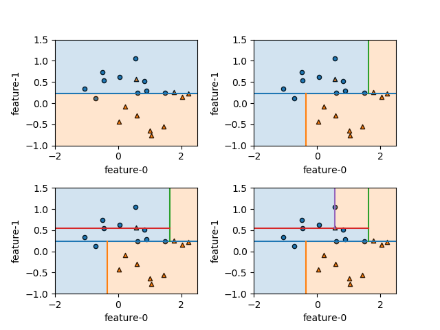
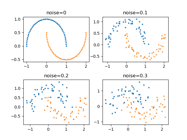
以下は、stop_levelを順次増やしていって、領域が分割される過程を描いた例。

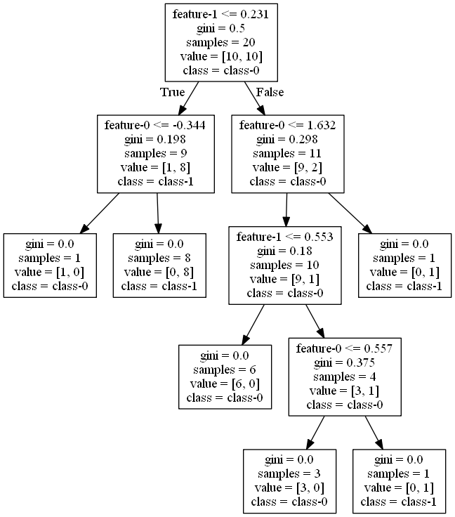
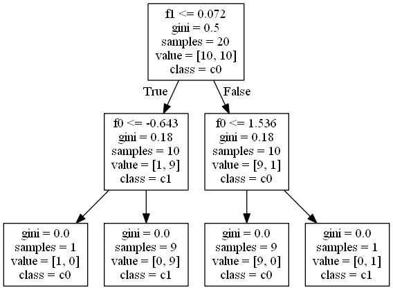
決定木のツリー表示

DecisionTreeClassificationオブジェクトを可視化する環境によって、決定木を表示する例。

環境構築
1. Pythonでpydotplusパッケージを導入
2. Graphviz環境を構築
実行
1. sklearn.tree.export_graphviz()で決定木のdotデータを得る
2. pydotplus.graph_from_dot_data()でDotオブジェクトを生成
3. write_png()などのメソッドでグラフを画像として書き出す

import numpy as np
import pydotplus as pdp
from sklearn.datasets import make_moons
from sklearn.tree import DecisionTreeClassifier, export_graphviz

X, y = make_moons(n_samples=20, noise=0.25, random_state=5)

treeclf = DecisionTreeClassifier(random_state=0)
treeclf.fit(X, y)

dot_data = export_graphviz(treeclf, max_depth=None,
    feature_names=["feature-0", "feature-1"],
    class_names=["class-0", "class-1"])
graph = pdp.graph_from_dot_data(dot_data)
graph.write_png("tree.png")

# C:...\atom\app-1.47.0

import numpy as np

import pydotplus as pdp

from sklearn.datasets import make_moons

from sklearn.tree import DecisionTreeClassifier, export_graphviz

X, y = make_moons(n_samples=20, noise=0.25, random_state=5)

treeclf = DecisionTreeClassifier(random_state=0)

treeclf.fit(X, y)

dot_data = export_graphviz(treeclf, max_depth=None,

feature_names=["feature-0", "feature-1"],

class_names=["class-0", "class-1"])

graph = pdp.graph_from_dot_data(dot_data)

graph.write_png("tree.png")

# C:...\atom\app-1.47.0

このコードはAtom上でコードを実行したため、Atomのディレクトリーに画像ファイルが書き出される。

決定木の分割の考え方

2020-05-30 / tau / コメントする

決定木の分割の考え方

決定木のデータを特性量によって分割するには、分割後のノードの状態ができるだけうまく分かれていることが必要となる。この「うまく分かれている」状態は、言い換えれば分割後のノード内のデータができるだけ「揃っている」ともいえる。たとえば2クラスの分類をする場合、ノード内に1つのクラスしか含まれていない場合は最も「純度が高い」状態であり、2つのクラスのデータが半分ずつ含まれている場合に最も「純度が低い」状態となる。

このような状態を定量的に表すのにエントロピーとジニ不純度という2つの考え方があるが、ここではそれらを確認する。

エントロピー（平均情報量）とジニ不純度

定義

クラスc = 1~Cに属するデータがノードtに属しており、各クラスごとのデータ数をn_c、データの総数をNとする。この場合、このノードの純度／不純度を表すのに、エントロピー（entropy、平均情報量）とジニ不純度（Gini impurity）という2つの考え方がある。ノードtのエントロピーをI_H(t)、ジニ不純度をI_G(t)と表すと、それぞれの定義は以下の通り。

(1) $\begin{align*} I_H(t) &= - \sum_{c=1}^C p_c(t) \log p_c(t) = - \sum_{c=1}^C \frac{n_c}{N} \log \frac{n_c}{N} \\ I_G(t) &= 1 - \sum_{c=1}^C p_c^2 = 1 - \sum_{c=1}^C \left( \frac{n_c}{N} \right)^2 \end{align*}$

エントロピーの対数の底は何でもいいが、分類するクラス数にすると最も高いエントロピーが1になって都合がよいようだ）。

ジニ不純度については次の表現の方が直感的にわかりやすい。

(2) $\begin{equation*} I_G(t) = \sum_{c=1}^C p_c (1 - p_c) \end{equation*}$

これを展開すると先のI_Gと同じ形になるが、この形だと関数形が上に凸でp_c = 0, 1でI_G = 0となることがわかる。

計算例

クラス数Cのデータについて、あるノード内のデータが全て同じクラスの場合、純度が高い／不純度が低い。

(3) $\begin{align*} I_H(t) &= - \frac{N}{N} \log_C \frac{N}{N} = 0 \\ I_G(t) &= 1 - \left( \frac{N}{N} \right)^2 = 0 \end{align*}$

ノード内で全てのクラスのデータが同じ数ずつある場合、純度が低い／不純度が高い。

(4) $\begin{align*} I_H(t) &= - C \cdot \frac{N/C}{N} \log_C \frac{N/C}{N} = - C \cdot \frac{1}{C} \log_C \frac{1}{C} = 1 \\ I_G(t) &= 1 - C \left( \frac{N/C}{N} \right)^2 = 1 - \frac{1}{C} \end{align*}$

分布

あるノード内にN個の2クラスデータがあり、クラス1のデータ数をnとする。このとき、クラス1のデータの発生率pに対するエントロピー、ジニ不純度の分布は以下のようになる。

(5) $\begin{align*} I_H(p; t) &= - \frac{n}{N} \log_2 \frac{n}{N} - \frac{N-n}{N} \log_2 \frac{N-n}{N} \\ &= -p \log_2 p - (1-p) \log_2 (1-p) \\ I_G(p; t) &= 1 - \left( \frac{n}{N} \right)^2 - \left( \frac{N-n}{N} \right)^2 \\ &= 1 - p^2 - (1-p)^2 \end{align*}$

これらをグラフ化したのが以下の図。p = 0.5で双方最大値をとり、エントロピーは1 、ジニ不純度は0.5。グラフの形状を比較するため、ジニ不純度を2倍した線も入れている。

import numpy as np
import matplotlib.pyplot as plt

eps = 1e-3
p = np.linspace(eps, 1 - eps)
Ih = -p * np.log2(p) - (1 - p) * np.log2(1 - p)
Ig = 1 - p**2 - (1 - p)**2

fig, ax = plt.subplots()

ax.plot(p, Ih, c='tab:blue', label="Entropy", clip_on=False)
ax.plot(p, Ig, c='tab:orange', label="Gini impurity")
ax.plot(p, Ig*2, c='tab:orange', ls='dashed', label="Gini doubled"
    , clip_on=False)

ax.set_xlim(0, 1)
ax.set_ylim(0, 1)
ax.set_xticks(np.linspace(0, 1, 11))
ax.set_yticks(np.linspace(0, 1, 11))
ax.grid(True)
ax.set_aspect('equal')
ax.legend()

plt.show()

import numpy as np

import matplotlib.pyplot as plt

eps = 1e-3

p = np.linspace(eps, 1 - eps)

Ih = -p * np.log2(p) - (1 - p) * np.log2(1 - p)

Ig = 1 - p**2 - (1 - p)**2

fig, ax = plt.subplots()

ax.plot(p, Ih, c='tab:blue', label="Entropy", clip_on=False)

ax.plot(p, Ig, c='tab:orange', label="Gini impurity")

ax.plot(p, Ig*2, c='tab:orange', ls='dashed', label="Gini doubled"

, clip_on=False)

ax.set_xlim(0, 1)

ax.set_ylim(0, 1)

ax.set_xticks(np.linspace(0, 1, 11))

ax.set_yticks(np.linspace(0, 1, 11))

ax.grid(True)

ax.set_aspect('equal')

ax.legend()

plt.show()

ノード分割の考え方～利得

親ノードを子ノードに分割するのに最も妥当な分割とするには、分割後の子ノードの純度ができるだけ高くなるような特徴量を探すことになる。ある特徴量について、親ノードから子ノードに分割したときにどれだけ純度が高くなったかを比較する量として、利得（情報利得、gain）が用いられる。

親ノードt_Pにc = 1~Cのクラスのデータがそれぞれn_cずつあるとする。このときの親ノードのエントロピーI_H(t_P)、ジニ不純度I_G(t_P)は式(1)で計算される。

まずエントロピーについて考える。ある特徴量fを定めると左右のノードのデータ分布が決まり、その時の左ノードt_L、右ノードt_Lのエントロピーが以下のように計算される。

(6) $\begin{align*} & I_H(t_L) = -p_c(t_L) \sum_{c=1}^C \log p_c(t_L) = - \sum_{c=1}^C \frac{n_c(t_L)}{N(t_L)} \log \frac{n_c(t_L)}{N(t_L)} \\ & I_H(t_R) = -p_c(t_R) \sum_{c=1}^C \log p_c(t_R) = - \sum_{c=1}^C \frac{n_c(t_R)}{N(t_R)} \log \frac{n_c(t_R)}{N(t_R)} \end{align*}$

このとき、それぞれのノードのエントロピーにノードの重みw_L, w_Rを掛け、これを親ノードのエントロピーから引いた量を利得（gain、情報利得）という。重みを各ノードのデータ数の比率とすると、利得は以下のように計算される。

(7) $\begin{align*} G_H(t_P, f) &= I_H(t_P) - w_L I_H(t_L) - w_R I_H(t_R) \\ &= I_H(t_P) - \frac{n_L}{N} I_H(t_L) - \frac{n_R}{N} I_H(t_R) \end{align*}$

ジニ不純度についても同様の計算ができる。

(8) $\begin{align*} G_G(t_P, f) &= I_G(t_P) - w_L I_G(t_L) - w_R I_G(t_R) \\ &= I_G(t_P) - \frac{n_L}{N} I_G(t_L) - \frac{n_R}{N} I_G(t_R) \end{align*}$

利得は、ある特徴量の値によって分割した後の状態が、分割前の状態に対してどれだけ純度が高くなったかを表す。

決定木のノードを分割するにあたっては、子ノードの純度ができるだけ高くなるように（エントロピー／ジニ不純度が小さくなるように）fを選ぶことになる。

簡単な例

特徴量が1つでデータ数が少ないケースで、利得の計算を確認してみる。

000111と並んでいる場合

クラス0、1がこのように並んでいるとき、左から境界を動かしていったときの左右のノードの不純度、利得について計算した結果は以下の通り。

IHP=1.0, IGP=0.5
[0][0 0 1 1 1]:
  IHL=-0.000, IHR= 0.971, G_H= 0.191
  IGL= 0.000, IGR= 0.480, G_G= 0.100
[0 0][0 1 1 1]:
  IHL=-0.000, IHR= 0.811, G_H= 0.459
  IGL= 0.000, IGR= 0.375, G_G= 0.250
[0 0 0][1 1 1]:
  IHL=-0.000, IHR= 0.000, G_H= 1.000
  IGL= 0.000, IGR= 0.000, G_G= 0.500
[0 0 0 1][1 1]:
  IHL= 0.811, IHR= 0.000, G_H= 0.459
  IGL= 0.375, IGR= 0.000, G_G= 0.250
[0 0 0 1 1][1]:
  IHL= 0.971, IHR= 0.000, G_H= 0.191
  IGL= 0.480, IGR= 0.000, G_G= 0.100

IHP=1.0, IGP=0.5

[0][0 0 1 1 1]:

IHL=-0.000, IHR= 0.971, G_H= 0.191

IGL= 0.000, IGR= 0.480, G_G= 0.100

[0 0][0 1 1 1]:

IHL=-0.000, IHR= 0.811, G_H= 0.459

IGL= 0.000, IGR= 0.375, G_G= 0.250

[0 0 0][1 1 1]:

IHL=-0.000, IHR= 0.000, G_H= 1.000

IGL= 0.000, IGR= 0.000, G_G= 0.500

[0 0 0 1][1 1]:

IHL= 0.811, IHR= 0.000, G_H= 0.459

IGL= 0.375, IGR= 0.000, G_G= 0.250

[0 0 0 1 1][1]:

IHL= 0.971, IHR= 0.000, G_H= 0.191

IGL= 0.480, IGR= 0.000, G_G= 0.100

この場合、当然のことながら真ん中でノードを分割することで2つのクラスがきれいに分かれ、利得もこれを表している。

00100111と並んでいる場合

今度は一部に他のクラスが紛れ込んでいる場合。左のクラス0の集団に1つだけクラス1のデータが含まれているときの挙動を確認する。

IHP=1.0, IGP=0.5
[0][0 1 0 0 1 1 1]:
  IHL=-0.000, IHR= 0.985, G_H= 0.138
  IGL= 0.000, IGR= 0.490, G_G= 0.071
[0 0][1 0 0 1 1 1]:
  IHL=-0.000, IHR= 0.918, G_H= 0.311
  IGL= 0.000, IGR= 0.444, G_G= 0.167
[0 0 1][0 0 1 1 1]:
  IHL= 0.918, IHR= 0.971, G_H= 0.049
  IGL= 0.444, IGR= 0.480, G_G= 0.033
[0 0 1 0][0 1 1 1]:
  IHL= 0.811, IHR= 0.811, G_H= 0.189
  IGL= 0.375, IGR= 0.375, G_G= 0.125
[0 0 1 0 0][1 1 1]:
  IHL= 0.722, IHR= 0.000, G_H= 0.549
  IGL= 0.320, IGR= 0.000, G_G= 0.300
[0 0 1 0 0 1][1 1]:
  IHL= 0.918, IHR= 0.000, G_H= 0.311
  IGL= 0.444, IGR= 0.000, G_G= 0.167
[0 0 1 0 0 1 1][1]:
  IHL= 0.985, IHR= 0.000, G_H= 0.138
  IGL= 0.490, IGR= 0.000, G_G= 0.071

IHP=1.0, IGP=0.5

[0][0 1 0 0 1 1 1]:

IHL=-0.000, IHR= 0.985, G_H= 0.138

IGL= 0.000, IGR= 0.490, G_G= 0.071

[0 0][1 0 0 1 1 1]:

IHL=-0.000, IHR= 0.918, G_H= 0.311

IGL= 0.000, IGR= 0.444, G_G= 0.167

[0 0 1][0 0 1 1 1]:

IHL= 0.918, IHR= 0.971, G_H= 0.049

IGL= 0.444, IGR= 0.480, G_G= 0.033

[0 0 1 0][0 1 1 1]:

IHL= 0.811, IHR= 0.811, G_H= 0.189

IGL= 0.375, IGR= 0.375, G_G= 0.125

[0 0 1 0 0][1 1 1]:

IHL= 0.722, IHR= 0.000, G_H= 0.549

IGL= 0.320, IGR= 0.000, G_G= 0.300

[0 0 1 0 0 1][1 1]:

IHL= 0.918, IHR= 0.000, G_H= 0.311

IGL= 0.444, IGR= 0.000, G_G= 0.167

[0 0 1 0 0 1 1][1]:

IHL= 0.985, IHR= 0.000, G_H= 0.138

IGL= 0.490, IGR= 0.000, G_G= 0.071

左から1つ目2つ目と境界を動かしていくと少しずつ利得が上昇するが、左側のノードにクラス1のデータが入ってきたところでその不純度が跳ね上がり、利得が下がる（8～10行目）。その後再び利得は上昇し、右側のデータがクラス1のみ3つとなった時に利得が最大となっている。このとき左側のノードにクラス1のデータが1つ含まれているが、他の4つのデータがクラスゼロと多いため、不純度は比較的低い。

利得が最大となる時でも、完全にクラスが分かれた時に比べて半分近くの利得だが、これはデータ数の多い左側に異なるクラスのデータが含まれているからと考えられる。

ここまでの計算に使ったコードは以下の通り。

import numpy as np

def impurity(node):
    N = node.size
    n0 = node[node==0].size
    n1 = node[node==1].size
    p0, p1 = n0 / N, n1 / N
    entropy = - (p0 * np.log2(p0) if p0 > 0 else 0) \
              - (p1 * np.log2(p1) if p1 > 0 else 0)
    gini = 1 - p0*p0 - p1*p1

    return entropy, gini

#node = np.array([0, 0, 0, 1, 1, 1])
node = np.array([0, 0, 1, 0, 0, 1, 1, 1])

IHP, IGP = impurity(node)
print("IHP={}, IGP={}".format(IHP, IGP))
for pos in range(1, node.size):
    node_left = node[0:pos]
    node_right = node[pos:node.size]
    node_text = "{}{}".format(node_left, node_right)
    IHL, IGL = impurity(node_left)
    IHR, IGR = impurity(node_right)
    wL = node_left.size / node.size
    wR = node_right.size / node.size
    GH = IHP - wL*IHL - wR*IHR
    GG = IGP - wL*IGL - wR*IGR
    print("{}:".format(node_text))
    print("  IHL={:6.3f}, IHR={:6.3f}, G_H={:6.3f}".format(IHL, IHR, GH))
    print("  IGL={:6.3f}, IGR={:6.3f}, G_G={:6.3f}".format(IGL, IGR, GG))

import numpy as np

def impurity(node):

N = node.size

n0 = node[node==0].size

n1 = node[node==1].size

p0, p1 = n0 / N, n1 / N

entropy = - (p0 * np.log2(p0) if p0 > 0 else 0) \

- (p1 * np.log2(p1) if p1 > 0 else 0)

gini = 1 - p0*p0 - p1*p1

return entropy, gini

#node = np.array([0, 0, 0, 1, 1, 1])

node = np.array([0, 0, 1, 0, 0, 1, 1, 1])

IHP, IGP = impurity(node)

print("IHP={}, IGP={}".format(IHP, IGP))

for pos in range(1, node.size):

node_left = node[0:pos]

node_right = node[pos:node.size]

node_text = "{}{}".format(node_left, node_right)

IHL, IGL = impurity(node_left)

IHR, IGR = impurity(node_right)

wL = node_left.size / node.size

wR = node_right.size / node.size

GH = IHP - wL*IHL - wR*IHR

GG = IGP - wL*IGL - wR*IGR

print("{}:".format(node_text))

print(" IHL={:6.3f}, IHR={:6.3f}, G_H={:6.3f}".format(IHL, IHR, GH))

print(" IGL={:6.3f}, IGR={:6.3f}, G_G={:6.3f}".format(IGL, IGR, GG))

pyplot – グラフの端が枠線で切れる

2020-05-30 / tau / コメントする

pyplotでグラフを描画したとき、軸の端の方でグラフが見切れてしまう。軸の外側も使って線や点をクリップせずに表示させるには、各グラフ描画の引数でclip_on=Falseを指定する。

import numpy as np
import matplotlib.pyplot as plt

x = np.linspace(-np.pi, np.pi, num=200)
ys = np.sin(3*x)
yc = np.sin(3*x - np.pi)

xp = [-np.pi, np.pi]
yp1 = [-1, 1]
yp2 = [1, -1]

fig, ax = plt.subplots()

ax.plot(x, ys, linewidth=4)
ax.plot(x, yc, linewidth=4, clip_on=False)

ax.scatter(xp, yp1, s=80)
ax.scatter(xp, yp2, s=80, clip_on=False)

ax.set_xlim(-np.pi, np.pi)
ax.set_ylim(-1, 1)

plt.show()

import numpy as np

import matplotlib.pyplot as plt

x = np.linspace(-np.pi, np.pi, num=200)

ys = np.sin(3*x)

yc = np.sin(3*x - np.pi)

xp = [-np.pi, np.pi]

yp1 = [-1, 1]

yp2 = [1, -1]

fig, ax = plt.subplots()

ax.plot(x, ys, linewidth=4)

ax.plot(x, yc, linewidth=4, clip_on=False)

ax.scatter(xp, yp1, s=80)

ax.scatter(xp, yp2, s=80, clip_on=False)

ax.set_xlim(-np.pi, np.pi)

ax.set_ylim(-1, 1)

plt.show()

DecisionTreeClassifierの可視化環境

2020-05-27 / tau / コメントする

概要

Pythonのscikit-learnで提供される決定木のクラス分類モデルDecisionTreeClassifierの実行結果を可視化する環境について。

Graphvizとgraphvizパッケージ

この方法は、決定木の画像がPDFとして生成され、デフォルトのPDFリーダーが自動的に起動して確認できる。画像ファイルを利用する場合、PDFから切り出すか、以下のpydotplusパッケージを利用する。

import graphviz
from sklearn.datasets import make_moons
from sklearn.tree import DecisionTreeClassifier, export_graphviz

X, y = make_moons(n_samples=20, noise=0.25, random_state=3)

treeclf = DecisionTreeClassifier(random_state=0)
treeclf.fit(X, y)

dot_data = export_graphviz(treeclf, out_file=None,
    feature_names=["f0", "f1"], class_names=["c0", "c1"])
graph = graphviz.Source(dot_data)
graph.render("image", view=True)

import graphviz

from sklearn.datasets import make_moons

from sklearn.tree import DecisionTreeClassifier, export_graphviz

X, y = make_moons(n_samples=20, noise=0.25, random_state=3)

treeclf = DecisionTreeClassifier(random_state=0)

treeclf.fit(X, y)

dot_data = export_graphviz(treeclf, out_file=None,

feature_names=["f0", "f1"], class_names=["c0", "c1"])

graph = graphviz.Source(dot_data)

graph.render("image", view=True)

Graphvizとpydotplosパッケージ

この方法は、決定木の画像がファイルとして生成・保存される。画像を確認するためにファイルが保存されたディレクトリでファイルを開く手順が必要になるが、得られたファイルをそのまま活用することができる。

pydotplusのインストール

pydotplusをインストールする。

> pip install pydotplus

1	> pip install pydotplus

これだけでは次のようなエラーが出る。

pydotplus.graphviz.InvocationException: GraphViz's executables not found

1	pydotplus.graphviz.InvocationException: GraphViz's executables not found

Graphvizのインストール

Graphvizのサイトから実行ファイル(msiファイル)をダウンロード、インストールする。

実行方法1：Graphvizの実行位置を指定

以下のコード例13行目のように、Graphvizの実行プログラムの位置を指定。

import pydotplus as pdp
from sklearn.datasets import make_moons
from sklearn.tree import DecisionTreeClassifier, export_graphviz

X, y = make_moons(n_samples=20, noise=0.25, random_state=3)

treeclf = DecisionTreeClassifier(random_state=0)
treeclf.fit(X, y)

dot_data = export_graphviz(treeclf, out_file=None,
    feature_names=["f0", "f1"], class_names=["c0", "c1"])
graph = pdp.graph_from_dot_data(dot_data)
graph.progs = {'dot': u"C:\\Program Files (x86)\\Graphviz2.38\\bin\\dot.exe"}
graph.write_png("graph.png")

import pydotplus as pdp

from sklearn.datasets import make_moons

from sklearn.tree import DecisionTreeClassifier, export_graphviz

X, y = make_moons(n_samples=20, noise=0.25, random_state=3)

treeclf = DecisionTreeClassifier(random_state=0)

treeclf.fit(X, y)

dot_data = export_graphviz(treeclf, out_file=None,

feature_names=["f0", "f1"], class_names=["c0", "c1"])

graph = pdp.graph_from_dot_data(dot_data)

graph.progs = {'dot': u"C:\\Program Files (x86)\\Graphviz2.38\\bin\\dot.exe"}

graph.write_png("graph.png")

実行方法2：Graphvizへのパスを環境変数に登録

環境変数に上記のGraphvizのパスを指定する。

デスクトップのPCアイコンを右クリック→プロパティ
システム・ウィンドウ→システムの詳細設定
システムのプロパティダイアログ→環境変数ボタン
環境変数ダイアログのシステム環境変数→Pathを指定して編集ボタン
環境変数名の編集ダイアログ→新規ボタン
Graphvizへのパス(例えばC:\Program Files (x86)\Graphviz2.38\bin\)を入力してOK
以下、各ダイアログでOK

環境変数を設定しておくと、毎回パスを指定しなくてよい。

import pydotplus as pdp
from sklearn.datasets import make_moons
from sklearn.tree import DecisionTreeClassifier, export_graphviz

X, y = make_moons(n_samples=20, noise=0.25, random_state=3)

treeclf = DecisionTreeClassifier(random_state=0)
treeclf.fit(X, y)

dot_data = export_graphviz(treeclf, out_file=None,
    feature_names=["f0", "f1"], class_names=["c0", "c1"])
graph = pdp.graph_from_dot_data(dot_data)
graph.write_png("graph.png")

import pydotplus as pdp

from sklearn.datasets import make_moons

from sklearn.tree import DecisionTreeClassifier, export_graphviz

X, y = make_moons(n_samples=20, noise=0.25, random_state=3)

treeclf = DecisionTreeClassifier(random_state=0)

treeclf.fit(X, y)

dot_data = export_graphviz(treeclf, out_file=None,

feature_names=["f0", "f1"], class_names=["c0", "c1"])

graph = pdp.graph_from_dot_data(dot_data)

graph.write_png("graph.png")

dtreeviz

dtreevizのインストール

dtreevizをインストールする。

> pip install dtreeviz

1	> pip install dtreeviz

実行方法

Graphvizの実行方法2で環境変数を追加。

from sklearn.datasets import make_moons
from sklearn.tree import DecisionTreeClassifier
from dtreeviz.trees import dtreeviz

X, y = make_moons(n_samples=20, noise=0.25, random_state=3)

treeclf = DecisionTreeClassifier(random_state=0)
treeclf.fit(X, y)

viz = dtreeviz(treeclf, X, y, target_name="Classes",
    feature_names=["f0", "f1"], class_names=["c0", "c1"])

viz.view()

from sklearn.datasets import make_moons

from sklearn.tree import DecisionTreeClassifier

from dtreeviz.trees import dtreeviz

X, y = make_moons(n_samples=20, noise=0.25, random_state=3)

treeclf = DecisionTreeClassifier(random_state=0)

treeclf.fit(X, y)

viz = dtreeviz(treeclf, X, y, target_name="Classes",

feature_names=["f0", "f1"], class_names=["c0", "c1"])

viz.view()

scikit-learn – make_moons

2020-05-24 / tau / コメントする

概要

sklearn.datasets.make_moons()はクラス分類のためのデータを生成する。上向き、下向きの弧が相互にかみ合う形で生成され、単純な直線では分離できないデータセットを提供する。クラス数は常に2クラス。

得られるデータの形式

2つの配列X, yが返され、配列Xは列が特徴量、行がレコードの2次元配列。ターゲットyはレコード数分のクラス属性値の整数。

from sklearn.datasets import make_moons

X, y = make_moons(n_samples=10, random_state=0)

print("X:\n{}".format(X))
print("y:{}".format(y))

# X:
# [[ 6.12323400e-17  1.00000000e+00]
#  [ 1.70710678e+00 -2.07106781e-01]
#  [-1.00000000e+00  1.22464680e-16]
#  [ 2.00000000e+00  5.00000000e-01]
#  [ 7.07106781e-01  7.07106781e-01]
#  [ 2.92893219e-01 -2.07106781e-01]
#  [ 1.00000000e+00 -5.00000000e-01]
#  [-7.07106781e-01  7.07106781e-01]
#  [ 1.00000000e+00  0.00000000e+00]
#  [ 0.00000000e+00  5.00000000e-01]]
# y:[0 1 0 1 0 1 1 0 0 1]

from sklearn.datasets import make_moons

X, y = make_moons(n_samples=10, random_state=0)

print("X:\n{}".format(X))

print("y:{}".format(y))

# X:

# [[ 6.12323400e-17 1.00000000e+00]

# [ 1.70710678e+00 -2.07106781e-01]

# [-1.00000000e+00 1.22464680e-16]

# [ 2.00000000e+00 5.00000000e-01]

# [ 7.07106781e-01 7.07106781e-01]

# [ 2.92893219e-01 -2.07106781e-01]

# [ 1.00000000e+00 -5.00000000e-01]

# [-7.07106781e-01 7.07106781e-01]

# [ 1.00000000e+00 0.00000000e+00]

# [ 0.00000000e+00 5.00000000e-01]]

# y:[0 1 0 1 0 1 1 0 0 1]

利用例

以下の例では、noiseパラメーターを変化させている。

import matplotlib.pyplot as plt
from sklearn.datasets import make_moons

noises = [0, 0.1, 0.2, 0.3]
fig, axs = plt.subplots(2, 2)
axs_1d = axs.reshape(axs.size)

for ax, noise in zip(axs_1d, noises):
    plt.subplots_adjust(hspace=0.4)
    X, y = make_moons(noise=noise, random_state=0)
    ax.scatter(X[y==0][:, 0], X[y==0][:, 1], s=5, marker='o')
    ax.scatter(X[y==1][:, 0], X[y==1][:, 1], s=5, marker='^')
    ax.set_title("noise={}".format(noise))

plt.show()

import matplotlib.pyplot as plt

from sklearn.datasets import make_moons

noises = [0, 0.1, 0.2, 0.3]

fig, axs = plt.subplots(2, 2)

axs_1d = axs.reshape(axs.size)

for ax, noise in zip(axs_1d, noises):

plt.subplots_adjust(hspace=0.4)

X, y = make_moons(noise=noise, random_state=0)

ax.scatter(X[y==0][:, 0], X[y==0][:, 1], s=5, marker='o')

ax.scatter(X[y==1][:, 0], X[y==1][:, 1], s=5, marker='^')

ax.set_title("noise={}".format(noise))

plt.show()

パラメーターの指定

sklearn.datasets.make_moons(n_samples=100, shuffle=True, noise=None, random_state=None)

1	sklearn.datasets.make_moons(n_samples=100, shuffle=True, noise=None, random_state=None)

n_samples

1つの数値で与えた場合は全データ数、2要素のタプルで与えた場合はそれぞれのクラスのデータ数。デフォルトは100。
shuffle: データをシャッフルするかどうか。デフォルトはTrue。
noise: データに加えられるノイズの標準偏差。デフォルトはノイズなし。
random_state: データ生成の乱数系列。

線形モデルによる多クラス分類

2020-05-23 / tau / 4件のコメント

概要

この項はO’REILLYの「Pythonではじめる機械学習」の「2.3.3.6　線形モデルによる多クラス分類」を自分なりに理解しやすいようにトレースしたもの。扱いやすい仮想のデータセットを生成し、LinearSVCモデルでこれらを分類する流れを例示している。

例えば特徴量x₁～x_nのデータxをC₁, C₂の2クラスに分類する線形モデルは以下とおり。

(1) $\begin{gather*} y = b + w_1 x_1 + \cdots + w_n x_n \\ \left\{ \begin{array}{ll} y \ge 0 \quad \rightarrow \quad \boldsymbol{x} \in C_1 \\ y < 0 \quad \rightarrow \quad \boldsymbol{x} \in C_2 \end{array} \right. \end{gather*}$

yの符号によってどちらのクラスに分類されるかを決定するが、1つの式で3つ以上のクラスを分類することはできない（ただし一般化線形モデル(GLM)であるLogistic回帰は多クラス分類が可能）。

このような2クラス分類を多クラス分類に拡張する方法の一つが1対その他(one-vs-rest, one-vs-the-rest, 1vR)という考え方で、1つの式によって、あるクラスとその他すべてのクラスを分けようというもの。この式の形は(1)と同じで、yの値は与えられたデータがそのクラスに属する確信度(confidence)を表す。クラスの数だけこの分類器(one-vs-the-rest-classifier)を準備し、あるデータが与えられたとき、最も確信度が高いクラスに属すると考える。たとえばn個の特徴量を持つデータの3クラス分類の場合、次のように3つの分類器を準備し、与えられたデータxはy_cの値が最も大きいクラスに属する。

(2) $\begin{gather*} y_0 = b_0 + w_{01} x_1 + \cdots + w_{0n} x_n \\ y_1 = b_1 + w_{11} x_1 + \cdots + w_{1n} x_n \\ y_2 = b_2 + w_{21} x_1 + \cdots + w_{2n} x_n \end{gather*}$

LinearSVCによる多クラス分類の例

データの準備

準備として、shikit-leran.datasetsのmake_blobs()で、2つの特徴量と3つのクラスのデータセットを生成する。

import numpy as np
import matplotlib.pyplot as plt
from sklearn.datasets import make_blobs

X, y = make_blobs(random_state=42)

fig, ax = plt.subplots()

f0_min, f0_max = -10, 8
f1_min, f1_max = -10, 15
markers = ['o', '^', 'v']

for cls, marker in zip(range(3), markers):
    x = X[y==cls]
    ax.scatter(x[:, 0], x[:, 1],
        ec='k', marker=marker, label="Class {}".format(cls))

ax.set_xlim(f0_min, f0_max)
ax.set_ylim(f1_min, f1_max)
ax.set_xlabel("Feature 0")
ax.set_ylabel("Feature 1")
ax.legend()

plt.show()

import numpy as np

import matplotlib.pyplot as plt

from sklearn.datasets import make_blobs

X, y = make_blobs(random_state=42)

fig, ax = plt.subplots()

f0_min, f0_max = -10, 8

f1_min, f1_max = -10, 15

markers = ['o', '^', 'v']

for cls, marker in zip(range(3), markers):

x = X[y==cls]

ax.scatter(x[:, 0], x[:, 1],

ec='k', marker=marker, label="Class {}".format(cls))

ax.set_xlim(f0_min, f0_max)

ax.set_ylim(f1_min, f1_max)

ax.set_xlabel("Feature 0")

ax.set_ylabel("Feature 1")

ax.legend()

plt.show()

LinearSVCによる学習

学習とモデルの形

scikit-learn.linear_modelのLinearSVC(Linear Support Vector Classification)は多クラス分類のモデルを提供する。このモデルをmake_blobs()で生成したデータで学習させると、3行2列の係数(LinearSVC.coef_)と3要素の切片(LinearSVC.intercept_)を得る。

import numpy as np
import matplotlib.pyplot as plt
from pandas import DataFrame
from sklearn.datasets import make_blobs
from sklearn.svm import LinearSVC

X, y = make_blobs(random_state=42)
df = DataFrame(X, columns=["f0", "f1"])
df['target'] = y

linsvm = LinearSVC().fit(X, y)
w = linsvm.coef_
b = linsvm.intercept_

print("Intercept: {}".format(b))
print("Coefficients(class, feature):\n{}".format(w))

# Intercept: [-1.07745476  0.13140569 -0.08604816]
# Coefficients(class, feature):
# [[-0.17491916  0.23140527]
#  [ 0.47621794 -0.06937226]
#  [-0.18914243 -0.20399679]]

import numpy as np

import matplotlib.pyplot as plt

from pandas import DataFrame

from sklearn.datasets import make_blobs

from sklearn.svm import LinearSVC

X, y = make_blobs(random_state=42)

df = DataFrame(X, columns=["f0", "f1"])

df['target'] = y

linsvm = LinearSVC().fit(X, y)

w = linsvm.coef_

b = linsvm.intercept_

print("Intercept: {}".format(b))

print("Coefficients(class, feature):\n{}".format(w))

# Intercept: [-1.07745476 0.13140569 -0.08604816]

# Coefficients(class, feature):

# [[-0.17491916 0.23140527]

# [ 0.47621794 -0.06937226]

# [-0.18914243 -0.20399679]]

これらの係数の行と切片の要素は分類されるべきクラス、係数の列は特徴量に対応している。クラスに対するインデックスをc = 0, 1, 2、特徴量f₀, f₁に対するインデックスをf= 0, 1とすると、上記の結果は以下のような意味になる。

(3) $\begin{align*} w_{cf} &= \left[ \begin{array}{rrr} -0.17492222 & 0.23140089 \\ 0.4762125 & -0.06936704 \\ -0.18914556 & -0.20399715 \end{array} \right] \\ b_c &= [-1.07745632 \quad 0.13140349 \quad -0.08604899] \end{align*}$

これらの係数、切片を用いたクラス分類の予測式は以下の通りで、LinearSVCではdecision function（決定関数）とされている。

(4) $\begin{equation*} y_c = b_c + w_{c0} \times f_0 + w_{c1} \times f_1 \end{equation*}$

あるデータの特徴量f₀, f₁に対して上記のy_cが正の時にはそのデータはクラスc、負の時にはクラスc以外であると判定される。

coef_やintercept_の値は、実行ごとにわずかに異なる（10⁻⁶くらいのオーダー）。LinearSVCのコンストラクターの引数にrandom_stateが含まれていて、ドキュメントに以下のような記述があった。

The underlying C implementation uses a random number generator to select features when fitting the model. It is thus not uncommon to have slightly different results for the same input data. If that happens, try with a smaller tol parameter.The underlying implementation, liblinear, uses a sparse internal representation for the data that will incur a memory copy.

Predict output may not match that of standalone liblinear in certain cases. See differences from liblinear in the narrative documentation.

訓練データに対する決定関数・確信度

データセットの100個の各データに対してy_c (c = 0, 1, 2)を計算した結果は以下の通り。

df['y0'] = b[0] + w[0, 0] * df['f0'] + w[0, 1] * df['f1']
df['y1'] = b[1] + w[1, 0] * df['f0'] + w[1, 1] * df['f1']
df['y2'] = b[2] + w[2, 0] * df['f0'] + w[2, 1] * df['f1']

print(df)

# DataFrame adding Confidences:
#           f0        f1  target        y0        y1        y2
# 0  -7.726421 -8.394957       2 -1.668593 -2.965677  3.087890
# 1   5.453396  0.742305       1 -1.859585  2.676915 -1.268945
# 2  -2.978672  9.556846       0  1.655077 -1.950071 -1.472221
# 3   6.042673  0.571319       1 -2.002228  2.969401 -1.345521
# 4  -6.521840 -6.319325       2 -1.398985 -2.536026  2.436631
# ..       ...       ...     ...       ...       ...       ...
# 95 -3.186120  9.625962       0  1.707357 -2.053656 -1.447083
# 96 -1.478198  9.945566       0  1.482567 -1.262485 -1.835322
# 97  4.478593  2.377221       1 -1.310745  2.099279 -1.418086
# 98 -5.796576 -5.826308       2 -1.411761 -2.224844  2.198878
# 99 -3.348415  8.705074       0  1.522647 -2.067060 -1.228528
# 
# [100 rows x 6 columns]

df['y0'] = b[0] + w[0, 0] * df['f0'] + w[0, 1] * df['f1']

df['y1'] = b[1] + w[1, 0] * df['f0'] + w[1, 1] * df['f1']

df['y2'] = b[2] + w[2, 0] * df['f0'] + w[2, 1] * df['f1']

print(df)

# DataFrame adding Confidences:

# f0 f1 target y0 y1 y2

# 0 -7.726421 -8.394957 2 -1.668593 -2.965677 3.087890

# 1 5.453396 0.742305 1 -1.859585 2.676915 -1.268945

# 2 -2.978672 9.556846 0 1.655077 -1.950071 -1.472221

# 3 6.042673 0.571319 1 -2.002228 2.969401 -1.345521

# 4 -6.521840 -6.319325 2 -1.398985 -2.536026 2.436631

# .. ... ... ... ... ... ...

# 95 -3.186120 9.625962 0 1.707357 -2.053656 -1.447083

# 96 -1.478198 9.945566 0 1.482567 -1.262485 -1.835322

# 97 4.478593 2.377221 1 -1.310745 2.099279 -1.418086

# 98 -5.796576 -5.826308 2 -1.411761 -2.224844 2.198878

# 99 -3.348415 8.705074 0 1.522647 -2.067060 -1.228528

# [100 rows x 6 columns]

たとえばNo.0のデータはクラス2に属するので確信度はy2が正となり、他の2つのクラスに対しては負の値になっている。

上の計算ではintercept_とcoef_を使ってもともとの決定関数の式から確信度を計算したが、LinearSVCのdecition_function()メソッドで同じ結果を得ることができる。たとえばNo.0～2のデータで計算してみると以下の通りで同じ結果。

print("decision_function values for first 3 data")
print(linsvm.decision_function(df.iloc[0:3, 0:2]))

# decision_function values for first 3 data
# [[-1.668593   -2.96567746  3.08789015]
#  [-1.85958483  2.67691534 -1.26894468]
#  [ 1.65507664 -1.95007141 -1.47222084]]

print("decision_function values for first 3 data")

print(linsvm.decision_function(df.iloc[0:3, 0:2]))

# decision_function values for first 3 data

# [[-1.668593 -2.96567746 3.08789015]

# [-1.85958483 2.67691534 -1.26894468]

# [ 1.65507664 -1.95007141 -1.47222084]]

テストデータに対する予測

3つのテストデータを用意してクラス分類をしてみる。

X_test = np.array([[4, -2], [-2, 2], [-6, 5]])
preds = linsvm.predict(X_test)
print("Prediction:")
for x_test, pred in zip(X_test, preds):
    print("{} -> {}".format(x_test, pred))
print()
print("Confidences of 3 points:\n{}".format(linsvm.decision_function(X_test)))

# Prediction:
# [ 4 -2] -> 1
# [-2  2] -> 2
# [-6  5] -> 0
# 
# Confidences of 3 points:
# [[-2.23994194  2.17502199 -0.43462432]
#  [-0.2648059  -0.95977473 -0.11575688]
#  [ 1.12908656 -3.07276329  0.02882249]]

X_test = np.array([[4, -2], [-2, 2], [-6, 5]])

preds = linsvm.predict(X_test)

print("Prediction:")

for x_test, pred in zip(X_test, preds):

print("{} -> {}".format(x_test, pred))

print()

print("Confidences of 3 points:\n{}".format(linsvm.decision_function(X_test)))

# Prediction:

# [ 4 -2] -> 1

# [-2 2] -> 2

# [-6 5] -> 0

# Confidences of 3 points:

# [[-2.23994194 2.17502199 -0.43462432]

# [-0.2648059 -0.95977473 -0.11575688]

# [ 1.12908656 -3.07276329 0.02882249]]

各データとも分類されたクラスに対応する確信度が最も高い。ただし2つ目のデータについては全てのクラスに対する確信度が負の値で、その中で最も値が大きいクラス2に分類されている。

これらを図示すると以下のようになり、クラス2に分類された▼のデータは確かにどのデータにも属していそうな位置にある。

以上のコードをまとめておく。

import numpy as np
import matplotlib.pyplot as plt
from pandas import DataFrame
from sklearn.datasets import make_blobs
from sklearn.svm import LinearSVC

X, y = make_blobs(random_state=42)
df = DataFrame(X, columns=["f0", "f1"])
df['target'] = y

linsvm = LinearSVC().fit(X, y)
w = linsvm.coef_
b = linsvm.intercept_

print("Intercept: {}".format(b))
print("Coefficients(class, feature):\n{}".format(w))

print()

df['y0'] = b[0] + w[0, 0] * df['f0'] + w[0, 1] * df['f1']
df['y1'] = b[1] + w[1, 0] * df['f0'] + w[1, 1] * df['f1']
df['y2'] = b[2] + w[2, 0] * df['f0'] + w[2, 1] * df['f1']

print("DataFrame adding Confidences:\n{}".format(df))

print()

print("decision_function values for first 3 data")
print(linsvm.decision_function(df.iloc[0:3, 0:2]))

print()

X_test = np.array([[4, -2], [-2, 2], [-6, 5]])
preds = linsvm.predict(X_test)
print("Prediction:")
for x_test, pred in zip(X_test, preds):
    print("{} -> {}".format(x_test, pred))
print()
print("Confidences of 3 points:\n{}".format(linsvm.decision_function(X_test)))

fig, ax = plt.subplots()

f0_min, f0_max = -10, 8
f1_min, f1_max = -10, 15
markers = ['o', '^', 'v']

for cls, marker in zip(range(3), markers):
    x = X[y==cls]
    ax.scatter(x[:, 0], x[:, 1],
        ec='k', marker=marker, label="Class {}".format(cls))

ax.scatter(X_test[0][0], X_test[0][1],
    ec='k', c='tab:orange', marker=markers[1], s=80)
ax.scatter(X_test[1][0], X_test[1][1],
    ec='k', c='tab:green', marker=markers[2], s=80)
ax.scatter(X_test[2][0], X_test[2][1],
    ec='k', c='tab:blue', marker=markers[0], s=80)

ax.set_xlim(f0_min, f0_max)
ax.set_ylim(f1_min, f1_max)
ax.set_xlabel("Feature 0")
ax.set_ylabel("Feature 1")
ax.legend()

plt.show()

import numpy as np

import matplotlib.pyplot as plt

from pandas import DataFrame

from sklearn.datasets import make_blobs

from sklearn.svm import LinearSVC

X, y = make_blobs(random_state=42)

df = DataFrame(X, columns=["f0", "f1"])

df['target'] = y

linsvm = LinearSVC().fit(X, y)

w = linsvm.coef_

b = linsvm.intercept_

print("Intercept: {}".format(b))

print("Coefficients(class, feature):\n{}".format(w))

print()

df['y0'] = b[0] + w[0, 0] * df['f0'] + w[0, 1] * df['f1']

df['y1'] = b[1] + w[1, 0] * df['f0'] + w[1, 1] * df['f1']

df['y2'] = b[2] + w[2, 0] * df['f0'] + w[2, 1] * df['f1']

print("DataFrame adding Confidences:\n{}".format(df))

print()

print("decision_function values for first 3 data")

print(linsvm.decision_function(df.iloc[0:3, 0:2]))

print()

X_test = np.array([[4, -2], [-2, 2], [-6, 5]])

preds = linsvm.predict(X_test)

print("Prediction:")

for x_test, pred in zip(X_test, preds):

print("{} -> {}".format(x_test, pred))

print()

print("Confidences of 3 points:\n{}".format(linsvm.decision_function(X_test)))

fig, ax = plt.subplots()

f0_min, f0_max = -10, 8

f1_min, f1_max = -10, 15

markers = ['o', '^', 'v']

for cls, marker in zip(range(3), markers):

x = X[y==cls]

ax.scatter(x[:, 0], x[:, 1],

ec='k', marker=marker, label="Class {}".format(cls))

ax.scatter(X_test[0][0], X_test[0][1],

ec='k', c='tab:orange', marker=markers[1], s=80)

ax.scatter(X_test[1][0], X_test[1][1],

ec='k', c='tab:green', marker=markers[2], s=80)

ax.scatter(X_test[2][0], X_test[2][1],

ec='k', c='tab:blue', marker=markers[0], s=80)

ax.set_xlim(f0_min, f0_max)

ax.set_ylim(f1_min, f1_max)

ax.set_xlabel("Feature 0")

ax.set_ylabel("Feature 1")

ax.legend()

plt.show()

LinearSVCの決定境界

クラスごとのone-vs-restの決定境界

blobsデータは明確に分かれた3つのクラスに分類され、それぞれに対する決定関数の切片と係数が得られた。そこで、各決定関数の決定関数の意思決定境界(decision boundary)を描いてみる。意思決定境界は決定関数の値がゼロとなる線なので、以下の式で表される。

(5) $\begin{gather*} b_c + w_0 f_0 + w_1 f_1 = 0 \quad \rightarrow \quad f_1 = \frac{-(b_c + w_{c0} f_0)}{w_{c1}} \end{gather*}$

3つの決定関数について決定境界を描いたのが以下の結果。

たとえばClass 0の実線は、Class 0の塊とその他(Class1, Class 2)の塊を1対その他で分けている。この線の上側では確信度はプラスで、下側ではマイナスとなっている。

import matplotlib.pyplot as plt
from pandas import DataFrame
from sklearn.datasets import make_blobs
from sklearn.svm import LinearSVC

f0_min, f0_max = -10, 8
f1_min, f1_max = -10, 15

X, y = make_blobs(random_state=42)
df = DataFrame(X, columns=["feature-0", "feature-1"])
df['target'] = y

linsvm = LinearSVC().fit(X, y)
w = linsvm.coef_
b = linsvm.intercept_

fig, ax = plt.subplots(figsize=(7.2, 4.8))

markers = ['o', '^', 'v']
line_styles = ['solid', 'dashed', 'dotted']

for c, marker, ls in zip(range(3), markers, line_styles):
    x = X[y==c]
    ax.scatter(x[:, 0], x[:, 1], marker=marker, label="Class {}".format(c))

    f1_left = -(b[c] + w[c, 0] * f0_min) / w[c, 1]
    f1_right = -(b[c] + w[c, 0] * f0_max) / w[c, 1]
    ax.plot([f0_min, f0_max], [f1_left, f1_right],
        linestyle=ls, linewidth=2, label="Class {}".format(c))

ax.set_xlim(f0_min, f0_max)
ax.set_ylim(f1_min, f1_max)
ax.legend(bbox_to_anchor=(1, 1))
fig.tight_layout()

plt.show()

import matplotlib.pyplot as plt

from pandas import DataFrame

from sklearn.datasets import make_blobs

from sklearn.svm import LinearSVC

f0_min, f0_max = -10, 8

f1_min, f1_max = -10, 15

X, y = make_blobs(random_state=42)

df = DataFrame(X, columns=["feature-0", "feature-1"])

df['target'] = y

linsvm = LinearSVC().fit(X, y)

w = linsvm.coef_

b = linsvm.intercept_

fig, ax = plt.subplots(figsize=(7.2, 4.8))

markers = ['o', '^', 'v']

line_styles = ['solid', 'dashed', 'dotted']

for c, marker, ls in zip(range(3), markers, line_styles):

x = X[y==c]

ax.scatter(x[:, 0], x[:, 1], marker=marker, label="Class {}".format(c))

f1_left = -(b[c] + w[c, 0] * f0_min) / w[c, 1]

f1_right = -(b[c] + w[c, 0] * f0_max) / w[c, 1]

ax.plot([f0_min, f0_max], [f1_left, f1_right],

linestyle=ls, linewidth=2, label="Class {}".format(c))

ax.set_xlim(f0_min, f0_max)

ax.set_ylim(f1_min, f1_max)

ax.legend(bbox_to_anchor=(1, 1))

fig.tight_layout()

plt.show()

全体を融合した決定境界

先の図の中で、各クラスの塊の近くでは、そのクラスの決定関数の値はプラスで他はマイナスとなっているが、真ん中の三角形の中や、その対角にある三角形の領域では、複数の確信度がマイナスあるいはプラスとなる。このような場合には、全クラスに対して着目するデータの決定関数値を計算し、その確信度が最も大きいクラスをそのデータのクラスラベルとして与える。

以下の図は、領域内の点について全て確信度を計算し、各点において最も確信度が大きいクラスをその点のクラスとして表現した図である。

各領域の境界が3つの決定関数から導かれた意思決定境界であり、その線上で決定関数の値が等しくなっている。

import numpy as np
import matplotlib.pyplot as plt
from pandas import DataFrame
from sklearn.datasets import make_blobs
from sklearn.svm import LinearSVC

f0_min, f0_max = -10, 8
f1_min, f1_max = -10, 15

X, y = make_blobs(random_state=42)
df = DataFrame(X, columns=["feature-0", "feature-1"])
df['target'] = y
n_classes = max(y + 1)

linsvm = LinearSVC().fit(X, y)
w = linsvm.coef_
b = linsvm.intercept_

markers = ['o', '^', 'v']
line_styles = ['solid', 'dashed', 'dotted']
colors = ['tab:blue', 'tab:orange', 'tab:green']

fig, ax = plt.subplots()

for f0 in np.linspace(f0_min, f0_max, 75):
    for f1 in np.linspace(f1_min, f1_max, 55):
        conf = [b[c] + w[c, 0] * f0 + w[c, 1] * f1 for c in range(n_classes)]
        ax.scatter(f0, f1, c=colors[np.argmax(conf)], marker='s', s=20, alpha=0.2)

for c, marker, ls in zip(range(3), markers, line_styles):
    x = X[y==c]
    ax.scatter(x[:, 0], x[:, 1], marker=marker, label="Class {}".format(c))

    f1_left = -(b[c] + w[c, 0] * f0_min) / w[c, 1]
    f1_right = -(b[c] + w[c, 0] * f0_max) / w[c, 1]
    ax.plot([f0_min, f0_max], [f1_left, f1_right], linestyle=ls, linewidth=2)

ax.set_xlim(f0_min, f0_max)
ax.set_ylim(f1_min, f1_max)
ax.legend()

plt.show()

import numpy as np

import matplotlib.pyplot as plt

from pandas import DataFrame

from sklearn.datasets import make_blobs

from sklearn.svm import LinearSVC

f0_min, f0_max = -10, 8

f1_min, f1_max = -10, 15

X, y = make_blobs(random_state=42)

df = DataFrame(X, columns=["feature-0", "feature-1"])

df['target'] = y

n_classes = max(y + 1)

linsvm = LinearSVC().fit(X, y)

w = linsvm.coef_

b = linsvm.intercept_

markers = ['o', '^', 'v']

line_styles = ['solid', 'dashed', 'dotted']

colors = ['tab:blue', 'tab:orange', 'tab:green']

fig, ax = plt.subplots()

for f0 in np.linspace(f0_min, f0_max, 75):

for f1 in np.linspace(f1_min, f1_max, 55):

conf = [b[c] + w[c, 0] * f0 + w[c, 1] * f1 for c in range(n_classes)]

ax.scatter(f0, f1, c=colors[np.argmax(conf)], marker='s', s=20, alpha=0.2)

for c, marker, ls in zip(range(3), markers, line_styles):

x = X[y==c]

ax.scatter(x[:, 0], x[:, 1], marker=marker, label="Class {}".format(c))

f1_left = -(b[c] + w[c, 0] * f0_min) / w[c, 1]

f1_right = -(b[c] + w[c, 0] * f0_max) / w[c, 1]

ax.plot([f0_min, f0_max], [f1_left, f1_right], linestyle=ls, linewidth=2)

ax.set_xlim(f0_min, f0_max)

ax.set_ylim(f1_min, f1_max)

ax.legend()

plt.show()

ndarray.reshape()の使い方

2020-05-23 / tau / コメントする

reshape()の考え方

a.reshape(d₁, ..., d_n)として変形する場合

n次元の配列になる
d₁ + ... + d_n = a.sizeでなければならない

要素が1つの場合

ndarrayの引数に1つの数値を指定するとndarrayクラスだが数値のように表示される。

import numpy as np

a = np.array(1)
print(a)
print(type(a))
print(a.size)
print(a * 2)

# 1
# <class 'numpy.ndarray'>
# 1
# 2

import numpy as np

a = np.array(1)

print(a)

print(type(a))

print(a.size)

print(a * 2)

# 1

# <class 'numpy.ndarray'>

# 1

# 2

これをreshape(1)とすると、1要素の1次元配列になる。

b = a.reshape(1)
print(b)

# [1]

b = a.reshape(1)

print(b)

# [1]

reshape(1, 1)とすると、1要素の2次元配列になる。reshape(1, 1, 1)なら3次元配列。

c = a.reshape(1, 1)
print(c)

d = a.reshape(1, 1, 1)
print(d)

# [[1]]
# [[[1]]]

c = a.reshape(1, 1)

print(c)

d = a.reshape(1, 1, 1)

print(d)

# [[1]]

# [[[1]]]

2次元化、3次元化された配列をreshape(1)とすると、1要素の1次元配列になる。

print(c.reshape(1))
print(d.reshape(1))

# [1]
# [1]

print(c.reshape(1))

print(d.reshape(1))

# [1]

1次元配列の変形

2次元1行の配列への変形

1次元配列をreshape(1, -1)とすると、その配列を要素とする2次元1行の配列になる。

import numpy as np

a = np.arange(4)
print(a)

b = a.reshape(1, -1)
print(b)

# [0 1 2 3]
# [[0 1 2 3]]

import numpy as np

a = np.arange(4)

print(a)

b = a.reshape(1, -1)

print(b)

# [0 1 2 3]

# [[0 1 2 3]]

2次元1列の配列への変形

1次元配列をreshape(-1, 1)とすると、その配列を要素とする2次元1列の配列となる。

c = a.reshape(-1, 1)
print(c)

# [[0]
#  [1]
#  [2]
#  [3]]

c = a.reshape(-1, 1)

print(c)

# [[0]

# [1]

# [2]

# [3]]

任意の次元の配列への変形

1次元配列をreshape(m, n)とすると、m行n列の2次元配列になる。m×nが配列のサイズと等しくないとエラーになる（いずれかを−1として自動設定させることは可能）。

d = a.reshape(2, 2)
print(d)

# [[0 1]
#  [2 3]]

d = a.reshape(2, 2)

print(d)

# [[0 1]

# [2 3]]

3次元以上の配列へも変形可能。

e = np.arange(12)
print(e)
print(e.reshape(2, 2, 3))

# [ 0  1  2  3  4  5  6  7  8  9 10 11]
# [[[ 0  1  2]
#   [ 3  4  5]]
# 
#  [[ 6  7  8]
#   [ 9 10 11]]]

e = np.arange(12)

print(e)

print(e.reshape(2, 2, 3))

# [ 0 1 2 3 4 5 6 7 8 9 10 11]

# [[[ 0 1 2]

# [ 3 4 5]]

# [[ 6 7 8]

# [ 9 10 11]]]

1次元配列への変換

任意の形状の配列aについてreshape(a.size)とすることで、1次元の配列に変換できる。

print(b.reshape(b.size))
print(c.reshape(c.size))
print(d.reshape(d.size))
print(e.reshape(e.size))

# [0 1 2 3]
# [0 1 2 3]
# [0 1 2 3]
# [ 0  1  2  3  4  5  6  7  8  9 10 11]

print(b.reshape(b.size))

print(c.reshape(c.size))

print(d.reshape(d.size))

print(e.reshape(e.size))

# [0 1 2 3]

# [ 0 1 2 3 4 5 6 7 8 9 10 11]

Python – itertools

2020-05-21 / tau / コメントする

概要

itertoolsは高速でメモリー効率のよいイテレーターを生成するツールを提供する。

主となる引数にはコレクション（リスト、タプル）を与える。

from itertools import cycle

for n, next in enumerate(cycle(['A', 'B', 'C'])):
    print(next, end='')
    if n == 6: break

# ABCABCA

from itertools import cycle

for n, next in enumerate(cycle(['A', 'B', 'C'])):

print(next, end='')

if n == 6: break

# ABCABCA

文字列を渡すと文字列中の1文字ずつを要素としたリストと同じ効果。

for n, next in enumerate(cycle("ABC")):
    print(next, end='')
    if n == 6: break

# ABCABCA

for n, next in enumerate(cycle("ABC")):

print(next, end='')

if n == 6: break

# ABCABCA

range()関数などコレクションを生成する対象も使える。

for n, next in enumerate(cycle(range(3))):
    print(next, end='')
    if n == 6: break

# 0120120

for n, next in enumerate(cycle(range(3))):

print(next, end='')

if n == 6: break

# 0120120

無限イテレーター(infinite iterators)

無限イテレーターは、コレクションの要素を繰り返し取り出し続ける。ループ処理に使う場合、break文などの終了処理が必要。

count()

itertools.count(start, [step]): startに与えた数値から初めてstepずつ増加させて取り出す。stepを省略した場合は1ずつ増やす。

for  n, digit in enumerate(count(3, 2)):
    print(digit, end=',')
    if n==5: break

# 3,5,7,9,11,13,

for n, digit in enumerate(count(3, 2)):

print(digit, end=',')

if n==5: break

# 3,5,7,9,11,13,

cycle()

itertools.cycle(p): コレクションpを与えて、その要素p0, p1, …, plastを取り出し、その後p0へ戻って繰り返す。

from itertools import cycle

for  n, digit in enumerate(cycle(range(4))):
    print(digit, end=',')
    if n==10: break

# 0,1,2,3,0,1,2,3,0,1,2,

from itertools import cycle

for n, digit in enumerate(cycle(range(4))):

print(digit, end=',')

if n==10: break

# 0,1,2,3,0,1,2,3,0,1,2,

repeat()

itertools.repeat(elem [, n]): elemで与えた要素を第2引数で与えた数値の回数分繰り返す。第2引数を省略すると無限回繰り返す。

for ch in repeat('Ha', 8):
    print(ch, end='')

# HaHaHaHaHaHaHaHa

for ch in repeat('Ha', 8):

print(ch, end='')

# HaHaHaHaHaHaHaHa

組み合わせイテレーター(combinatoric iterator)

組み合わせイテレーターは、コレクションの要素から指定した数を取り出し、それらの直積、順列、組み合わせを結果とする。

product()

itertools.product(p [, repeat=n]): コレクションpの要素について、repeatで指定した数の直積の結果をタプルで返す。同一の要素、順番の異なる同じ組み合わせの要素を持つ結果を許す。; 第2引数repeatを省略すると要素数1のタプルを返す。

from itertools import product

for str in product(['A', 'B', 'C'], repeat=2):
    print(str, end='')

print()

for str in product(['A', 'B', 'C']):
    print(str, end='')

# ('A', 'A')('A', 'B')('A', 'C')('B', 'A')('B', 'B')('B', 'C')('C', 'A')('C', 'B')('C', 'C')
# ('A',)('B',)('C',)

from itertools import product

for str in product(['A', 'B', 'C'], repeat=2):

print(str, end='')

print()

for str in product(['A', 'B', 'C']):

print(str, end='')

# ('A', 'A')('A', 'B')('A', 'C')('B', 'A')('B', 'B')('B', 'C')('C', 'A')('C', 'B')('C', 'C')

# ('A',)('B',)('C',)

permutations

itertools.permutations（p [, r=n]）: コレクションpの要素について、rで指定した数の順列の結果をタプルで返す。統一要素の組はなく、同じ組み合わせの要素の順番が異なる結果は許す。; 第2引数はrepeatではなくrである点に注意。rを省略すると、全ての要素に対する組み合わせを返す。

from itertools import permutations

for str in permutations("ABC", r=2):
    print(str, end='')

print()

for str in permutations("ABC"):
    print(str, end='')

# ('A', 'B')('A', 'C')('B', 'A')('B', 'C')('C', 'A')('C', 'B')
# ('A', 'B', 'C')('A', 'C', 'B')('B', 'A', 'C')('B', 'C', 'A')('C', 'A', 'B')('C', 'B', 'A')

from itertools import permutations

for str in permutations("ABC", r=2):

print(str, end='')

print()

for str in permutations("ABC"):

print(str, end='')

# ('A', 'B')('A', 'C')('B', 'A')('B', 'C')('C', 'A')('C', 'B')

# ('A', 'B', 'C')('A', 'C', 'B')('B', 'A', 'C')('B', 'C', 'A')('C', 'A', 'B')('C', 'B', 'A')

combinations

itertools.combinations(p, repeat=n): コレクションpの要素について、repeatで指定した数の組み合わせの結果をタプルで返す。同一要素の組はなく、同じ組み合わせで順番が異なるものは同じ結果となる。; 第2引数rは省略できない。省略するとそれ以降の実行がされないなど動作が不定になる。

from itertools import combinations

for str in combinations("ABC", r=2):
    print(str, end='')

# ('A', 'B')('A', 'C')('B', 'C'),

from itertools import combinations

for str in combinations("ABC", r=2):

print(str, end='')

# ('A', 'B')('A', 'C')('B', 'C'),

combinations_with_replacement

itertools.combinations_with_replacement(iterable, r)

組み合わせに、同一要素の重複を許す。

第2引数rは省略できない。省略するとそれ以降の実行がされないなど動作が不定になる。

from itertools import combinations

for str in combinations("ABC", r=2):
    print(str, end='')

# ('A', 'A')('A', 'B')('A', 'C')('B', 'B')('B', 'C')('C', 'C')

from itertools import combinations

for str in combinations("ABC", r=2):

print(str, end='')

# ('A', 'A')('A', 'B')('A', 'C')('B', 'B')('B', 'C')('C', 'C')

特に役立ちそうなもの

chain～リストの結合に使える

itertools.chain(*iterables): 複数のiterableを与え、それらの内容を並べた1つのイテレーターを返す。引数の先頭の'*'は複数のiterablesを展開したものであることを表す。

戻り値はイテレーターオブジェクト。

from itertools import chain

print(chain([0, 1, 2, 3], [4, 5]))

# <itertools.chain object at 0x028081B0>

from itertools import chain

print(chain([0, 1, 2, 3], [4, 5]))

# <itertools.chain object at 0x028081B0>

list()関数でリスト化すると、展開されたリストが得られる。

print(list(chain([0, 1, 2, 3], [4, 5])))

# [0, 1, 2, 3, 4, 5]

print(list(chain([0, 1, 2, 3], [4, 5])))

# [0, 1, 2, 3, 4, 5]

引数にはRangeのようなイテレーターも混在可能。

print(list(chain(range(3), [3, 4, 5])))

# [0, 1, 2, 3, 4, 5]

print(list(chain(range(3), [3, 4, 5])))

# [0, 1, 2, 3, 4, 5]

蛇足だが単一のiteratableはそのまま返されるだけ。

print(list(chain([0, 1, 2, 3, 4, 5])))

# [0, 1, 2, 3, 4, 5]

print(list(chain([0, 1, 2, 3, 4, 5])))

# [0, 1, 2, 3, 4, 5]

chain.from_iterabble～2次元リストの展開に

itertools.chain.from_iterable(iterables): 複数のiterableを与え、それらの内容を並べた1つのイテレーターを返す。引数の先頭に’*’がないのは、引数がiterableを要素に持つiterableであることを表す。

たとえば複数のリストを含む2次元リストの全要素を1次元に展開可能。from_iterable()はchainのコンストラクターの一つであり、モジュールのインポート方法とコンストラクターの呼び方に注意。

from itertools import chain

print(list(chain.from_iterable([[0], [1, 2], [3, 4, 5]])))

# [0, 1, 2, 3, 4, 5]

from itertools import chain

print(list(chain.from_iterable([[0], [1, 2], [3, 4, 5]])))

# [0, 1, 2, 3, 4, 5]

1次元リストは要素がiterableでないのでエラー。

print(list(chain.from_iterable([0, 1, 2])))

# TypeError: 'int' object is not iterable

print(list(chain.from_iterable([0, 1, 2])))

# TypeError: 'int' object is not iterable

ndarrayを要素とするリストは、要素の配列が展開されて1次元リストに。

print(list(chain.from_iterable([np.array([1]), np.array([2, 3])])))

# [1, 2, 3]

print(list(chain.from_iterable([np.array([1]), np.array([2, 3])])))

# [1, 2, 3]

ndarrayの2次元配列も展開可能。結果をリストでほしいときはlist()関数、配列でほしいときは一旦list()関数でリスト化してからnumpy.array()で配列化。

ary = np.array([[1, 2], [3, 4]])
print(ary)
# [[1 2]
#  [3 4]]

print(list(chain.from_iterable(ary)))
# [1, 2, 3, 4]

print(np.array(list(chain.from_iterable(ary))))
# [1 2 3 4]

ary = np.array([[1, 2], [3, 4]])

print(ary)

# [[1 2]

# [3 4]]

print(list(chain.from_iterable(ary)))

# [1, 2, 3, 4]

print(np.array(list(chain.from_iterable(ary))))

# [1 2 3 4]

zip_longest～最長の引数に合わせるzip

itertools.zip_longest(*iterables, fillvalue=None): 複数のiterableを与え、それらを先頭から順にまとめたイテレーターを返す。結果は最も長いiterableに合わせられ、足りない値はfillvalueで埋められる。

from itertools import zip_longest

iterable1 = "ABCDE"
iterable2 = [1, 2, 3]

for item1, item2 in zip_longest(iterable1, iterable2):
    print(item1, item2)
# A 1
# B 2
# C 3
# D None
# E None

for item1, item2 in zip_longest(iterable1, iterable2, fillvalue=0):
    print(item1, item2)
# A 1
# B 2
# C 3
# D 0
# E 0

from itertools import zip_longest

iterable1 = "ABCDE"

iterable2 = [1, 2, 3]

for item1, item2 in zip_longest(iterable1, iterable2):

print(item1, item2)

# A 1

# B 2

# C 3

# D None

# E None

for item1, item2 in zip_longest(iterable1, iterable2, fillvalue=0):

print(item1, item2)

# A 1

# B 2

# C 3

# D 0

# E 0

scikit-learn – make_blobs

2020-05-18 / tau / コメントする

概要

sklearn.datasets.make_blobls()は、クラス分類のためのデータを生成する。blobとはインクの染みなどを指し、散布図の点の様子からつけられてるようだ。

標準では、データの総数、特徴量の数、クラスターの数などを指定して実行し、特徴量配列X、ターゲットとなるクラスデータyのタプルが返される（引数の指定によってはもう1つ戻り値が追加される）。

得られるデータの形式

特徴量配列Xは列が特徴量、行がレコードの2次元配列。ターゲットyはレコード数分のクラス属性値の整数。

from sklearn.datasets import make_blobs

X, y = make_blobs(n_samples=10, random_state=0)

print(X)
print(y)

# [[ 1.12031365  5.75806083]
#  [ 1.7373078   4.42546234]
#  [ 2.36833522  0.04356792]
#  [ 0.87305123  4.71438583]
#  [-0.66246781  2.17571724]
#  [ 0.74285061  1.46351659]
#  [-4.07989383  3.57150086]
#  [ 3.54934659  0.6925054 ]
#  [ 2.49913075  1.23133799]
#  [ 1.9263585   4.15243012]]
# [0 0 1 0 2 2 2 1 1 0]

from sklearn.datasets import make_blobs

X, y = make_blobs(n_samples=10, random_state=0)

print(X)

print(y)

# [[ 1.12031365 5.75806083]

# [ 1.7373078 4.42546234]

# [ 2.36833522 0.04356792]

# [ 0.87305123 4.71438583]

# [-0.66246781 2.17571724]

# [ 0.74285061 1.46351659]

# [-4.07989383 3.57150086]

# [ 3.54934659 0.6925054 ]

# [ 2.49913075 1.23133799]

# [ 1.9263585 4.15243012]]

# [0 0 1 0 2 2 2 1 1 0]

利用例

そのままscikit-learnのモデルの入力とする。

from sklearn.datasets import make_blobs
from sklearn.model_selection import train_test_split
from sklearn.neighbors import KNeighborsClassifier

X, y = make_blobs(n_samples=100, centers=2, random_state=0)

X_train, X_test, y_train, y_test = train_test_split(X, y, random_state=0)

clf = KNeighborsClassifier(n_neighbors=1)
clf.fit(X_train, y_train)

print(clf.score(X_train, y_train))
print(clf.score(X_test, y_test))
# 1.0
# 0.96

from sklearn.datasets import make_blobs

from sklearn.model_selection import train_test_split

from sklearn.neighbors import KNeighborsClassifier

X, y = make_blobs(n_samples=100, centers=2, random_state=0)

X_train, X_test, y_train, y_test = train_test_split(X, y, random_state=0)

clf = KNeighborsClassifier(n_neighbors=1)

clf.fit(X_train, y_train)

print(clf.score(X_train, y_train))

print(clf.score(X_test, y_test))

# 1.0

# 0.96

クラスごとに色やマークを変えて散布図を描く。

import numpy as np
import matplotlib.pyplot as plt
from sklearn.datasets import make_blobs

X, y = make_blobs(n_samples=30, centers=3, random_state=10)

markers = ['o', '^', 'v']
fig, ax = plt.subplots()

for cluster, marker in zip(range(3), markers):
    x = X[y==cluster]
    ax.scatter(x[:, 0], x[:, 1], marker=marker)

plt.show()

import numpy as np

import matplotlib.pyplot as plt

from sklearn.datasets import make_blobs

X, y = make_blobs(n_samples=30, centers=3, random_state=10)

markers = ['o', '^', 'v']

fig, ax = plt.subplots()

for cluster, marker in zip(range(3), markers):

x = X[y==cluster]

ax.scatter(x[:, 0], x[:, 1], marker=marker)

plt.show()

パラメーターの指定

make_blobs(n_samples, n_features, centers, cluster_std,
           center_box, shuffle, random_state, return_centers)

1 2	make_blobs(n_samples, n_features, centers, cluster_std, center_box, shuffle, random_state, return_centers)

主なもの。

n_samples: 整数で指定した場合、生成されるサンプルの総数で戻り値Xの行数になる。配列で指定した場合、その要素数がクラスターの数となり、各要素はクラスターのデータ数となる。デフォルトは100。
n_features: 特徴量の数で、戻り値Xの列数になる。デフォルトは2
centers: クラスター中心の数。n_samplesを整数で指定してcentersを指定しない場合（デフォルトのNoneの場合）、centers=3となる。n_samplesを配列で指定した場合はNoneか[n_centers, n_features]の配列。
center_std: クラスターの標準偏差。

Logistic回帰～cancer～Pythonではじめる機械学習より

2020-05-17 / tau / コメントする

モデルの精度

breast_cancerデータセットに対してLogistic回帰モデル、scikit-learnのLogisticRegression適用し、訓練データとテストデータのスコアを計算してみる。

from sklearn.datasets import load_breast_cancer
from sklearn.model_selection import train_test_split
from sklearn.linear_model import LogisticRegression

ds = load_breast_cancer()

X_train, X_test, y_train, y_test = train_test_split(
    ds.data, ds.target, stratify=ds.target, random_state=42)

logreg = LogisticRegression().fit(X_train, y_train)
print("")
print("Training score: {}".format(logreg.score(X_train, y_train)))
print("Test score    : {}".format(logreg.score(X_test, y_test)))

# Training score: 0.9530516431924883
# Test score    : 0.958041958041958

from sklearn.datasets import load_breast_cancer

from sklearn.model_selection import train_test_split

from sklearn.linear_model import LogisticRegression

ds = load_breast_cancer()

X_train, X_test, y_train, y_test = train_test_split(

ds.data, ds.target, stratify=ds.target, random_state=42)

logreg = LogisticRegression().fit(X_train, y_train)

print("")

print("Training score: {}".format(logreg.score(X_train, y_train)))

print("Test score : {}".format(logreg.score(X_test, y_test)))

# Training score: 0.9530516431924883

# Test score : 0.958041958041958

（注）solverに関する警告と計算結果

上のコードを実行したとき、結果は書籍と整合しているが、警告表示が出た

...FutureWarning: Default solver will be changed to 'lbfgs' in 0.22. Specify a solver to silence this warning.
  FutureWarning)
Training score: 0.9530516431924883
Test score    : 0.958041958041958

...FutureWarning: Default solver will be changed to 'lbfgs' in 0.22. Specify a solver to silence this warning.

FutureWarning)

Training score: 0.9530516431924883

Test score : 0.958041958041958

この時点でscikit-learnのバージョンが古く(0.21.3)、将来のデフォルトが変更されるとのこと。そこでインスタンス生成時にデフォルトのソルバーを明示的にsolver='liblinear'と指定して実行すると、警告は出ず値もそのまま。

なお、solver='lbfgs'としてみたところ、計算が収束しない旨の警告が出た。

logreg = LogisticRegression(solver='lbfgs').fit(X_train, y_train)

1	logreg = LogisticRegression(solver='lbfgs').fit(X_train, y_train)

...ConvergenceWarning: lbfgs failed to converge. Increase the number of iterations.
  "of iterations.", ConvergenceWarning)
Training score: 0.9483568075117371
Test score    : 0.951048951048951

...ConvergenceWarning: lbfgs failed to converge. Increase the number of iterations.

"of iterations.", ConvergenceWarning)

Training score: 0.9483568075117371

Test score : 0.951048951048951

そこで収束回数を増やしていったところ、最大回数2000では収束せず、3000で収束し、警告は出なくなった。

logreg = LogisticRegression(solver='lbfgs', max_iter=3000).fit(X_train, y_train)

1	logreg = LogisticRegression(solver='lbfgs', max_iter=3000).fit(X_train, y_train)

Training score: 0.9577464788732394
Test score    : 0.958041958041958

1 2	Training score: 0.9577464788732394 Test score : 0.958041958041958

その後、scikit-learnのバージョンを0.23.0にアップグレードしたところ、デフォルトで警告は表示されず、収束回数に関する警告が同じように出て、結果も再現された。以下、ソルバーとしてliblinearを明示的に指定し、random_stateの値も書籍と同じ値として確認する。

学習精度の向上

先のC=1.0とliblinearによるスコアは、訓練データに対して0.953、テストデータに対して0.958と両方に対して高い値となっている。ここで、訓練データとテストデータのスコアが近いということは、適合不足の可能性がある。そこでC=100と値を大きくして、より柔軟なモデルにしてみる（柔軟なモデルとは、正則化を弱めて訓練データによりフィットしやすくしたモデル）。

logreg100 = LogisticRegression(C=100, solver='liblinear').fit(X_train, y_train)
print("Training score: {}".format(logreg100.score(X_train, y_train)))
print("Test score    : {}".format(logreg100.score(X_test, y_test)))

# Training score: 0.9788732394366197
# Test score    : 0.965034965034965

logreg100 = LogisticRegression(C=100, solver='liblinear').fit(X_train, y_train)

print("Training score: {}".format(logreg100.score(X_train, y_train)))

print("Test score : {}".format(logreg100.score(X_test, y_test)))

# Training score: 0.9788732394366197

# Test score : 0.965034965034965

訓練データ、テストデータともそれぞれ若干向上している。なお、Cの値を1000、10000ともっと大きくしてもスコアはほとんど変わらない。

今度は逆に、Cの値を1.0より小さくして正則化を強めてみると、訓練データ、テストデータ両方に対するスコアが下がってしまう。

logreg001 = LogisticRegression(C=0.01, solver='liblinear').fit(X_train, y_train)
print("Training score: {}".format(logreg001.score(X_train, y_train)))
print("Test score    : {}".format(logreg001.score(X_test, y_test)))

# Training score: 0.9342723004694836
# Test score    : 0.9300699300699301

logreg001 = LogisticRegression(C=0.01, solver='liblinear').fit(X_train, y_train)

print("Training score: {}".format(logreg001.score(X_train, y_train)))

print("Test score : {}".format(logreg001.score(X_test, y_test)))

# Training score: 0.9342723004694836

# Test score : 0.9300699300699301

Cを変化させたときの学習率曲線は以下の通り。Cが10より小さいところでは正則化が強く学習不足、そこを超えると学習率が頭打ちで、学習率の改善はそれほど顕著ではない。Logistic回帰モデルの学習率曲線のバリエーションについては、こちらでまとめている。

import numpy as np
import matplotlib.pyplot as plt
from sklearn.datasets import load_breast_cancer
from sklearn.model_selection import train_test_split
from sklearn.linear_model import LogisticRegression

C_pow_min = -4
C_pow_max = 3
C_pow_num = 100
Cs_pows = np.linspace(C_pow_min, C_pow_max, C_pow_num)
Cs = 10**Cs_pows

ds = load_breast_cancer()

X_train, X_test, y_train, y_test = train_test_split(
    ds.data, ds.target, stratify=ds.target, random_state=42)

fig, ax = plt.subplots()

score_trains = np.empty(0)
score_tests = np.empty(0)

for C in Cs:
    logreg = LogisticRegression(C=C, solver='liblinear').fit(X_train, y_train)
    score_trains = np.append(score_trains, logreg.score(X_train, y_train))
    score_tests = np.append(score_tests, logreg.score(X_test, y_test))

ax.plot(Cs, score_trains, label="Training")
ax.plot(Cs, score_tests, label="Test")

ax.set_xscale('log')
ax.legend()

plt.show()

import numpy as np

import matplotlib.pyplot as plt

from sklearn.datasets import load_breast_cancer

from sklearn.model_selection import train_test_split

from sklearn.linear_model import LogisticRegression

C_pow_min = -4

C_pow_max = 3

C_pow_num = 100

Cs_pows = np.linspace(C_pow_min, C_pow_max, C_pow_num)

Cs = 10**Cs_pows

ds = load_breast_cancer()

X_train, X_test, y_train, y_test = train_test_split(

ds.data, ds.target, stratify=ds.target, random_state=42)

fig, ax = plt.subplots()

score_trains = np.empty(0)

score_tests = np.empty(0)

for C in Cs:

logreg = LogisticRegression(C=C, solver='liblinear').fit(X_train, y_train)

score_trains = np.append(score_trains, logreg.score(X_train, y_train))

score_tests = np.append(score_tests, logreg.score(X_test, y_test))

ax.plot(Cs, score_trains, label="Training")

ax.plot(Cs, score_tests, label="Test")

ax.set_xscale('log')

ax.legend()

plt.show()

特徴量の係数

L2正則化の場合

breast_cancerデータセットに対してLogisticRegressionを学習させた場合の、30個の特徴量に対する係数をプロットする。liblinearソルバーで、デフォルトでL2正則化を行っている。Cの値が大きいほど正則化の効果が弱く、係数の絶対値が大きくなっている。

書籍で注意喚起しているのは3番目の特徴量mean perimeterで、モデルによって正負が入れ替わることから、クラス分類に対する信頼性を問題にしている。

ここで書籍について以下の点が気になった。

logreg001のインスタンス生成時にC=0.01としているが、凡例で”C=0.001″としている（グラフの結果はあまり変わらない）
logreg100でC=100とすると、書籍にあるような結果にならない（worst concave pointsが-8以下になるなど、分布が大幅に変わってくる）
C=20とすると、概ね書籍と同じ分布になる（若干異なる部分は残る）

いずれにしても”Pythonではじめる機械学習”は、入門者にとってとてもありがたいきっかけを提供してくれる良著であることに変わりはない。

import numpy as np
import matplotlib.pyplot as plt
import matplotlib.patches as pch
from sklearn.datasets import load_breast_cancer
from sklearn.model_selection import train_test_split
from sklearn.linear_model import LogisticRegression

ds = load_breast_cancer()

X_train, X_test, y_train, y_test = train_test_split(
    ds.data, ds.target, stratify=ds.target, random_state=42)

logreg1 = LogisticRegression(solver='liblinear').fit(X_train, y_train)
logreg20 = LogisticRegression(C=20, solver='liblinear').fit(X_train, y_train)
logreg001 = LogisticRegression(C=0.01, solver='liblinear').fit(X_train, y_train)

x_scatter = np.linspace(0, 1, len(ds.feature_names))

fig, ax = plt.subplots(figsize=(6.4, 6.4))

ax.scatter(x_scatter, logreg1.coef_, marker='o', c='grey', s=100,
    label="C=1.0")
ax.scatter(x_scatter, logreg001.coef_, marker='1', c='blue', s=100,
    label="C=0.01")
ax.scatter(x_scatter, logreg20.coef_, marker='2', c='red', s = 100,
    label="C=20")
ax.plot([0, 1], [0, 0], c='k', zorder=-100)
ax.add_patch(pch.Arrow(2/30, -4, 0, 3, width=1/30))

ax.set_xticks(x_scatter)
ax.set_xticklabels(ds.feature_names, rotation=90)
ax.set_xlim(0, 1)
ax.legend()

fig.subplots_adjust(bottom=0.3)

plt.show()

import numpy as np

import matplotlib.pyplot as plt

import matplotlib.patches as pch

from sklearn.datasets import load_breast_cancer

from sklearn.model_selection import train_test_split

from sklearn.linear_model import LogisticRegression

ds = load_breast_cancer()

X_train, X_test, y_train, y_test = train_test_split(

ds.data, ds.target, stratify=ds.target, random_state=42)

logreg1 = LogisticRegression(solver='liblinear').fit(X_train, y_train)

logreg20 = LogisticRegression(C=20, solver='liblinear').fit(X_train, y_train)

logreg001 = LogisticRegression(C=0.01, solver='liblinear').fit(X_train, y_train)

x_scatter = np.linspace(0, 1, len(ds.feature_names))

fig, ax = plt.subplots(figsize=(6.4, 6.4))

ax.scatter(x_scatter, logreg1.coef_, marker='o', c='grey', s=100,

label="C=1.0")

ax.scatter(x_scatter, logreg001.coef_, marker='1', c='blue', s=100,

label="C=0.01")

ax.scatter(x_scatter, logreg20.coef_, marker='2', c='red', s = 100,

label="C=20")

ax.plot([0, 1], [0, 0], c='k', zorder=-100)

ax.add_patch(pch.Arrow(2/30, -4, 0, 3, width=1/30))

ax.set_xticks(x_scatter)

ax.set_xticklabels(ds.feature_names, rotation=90)

ax.set_xlim(0, 1)

ax.legend()

fig.subplots_adjust(bottom=0.3)

plt.show()

L1正則化の場合

ソルバーを同じliblinearとして、penalty='l1'と明示的に指定する。今回はL2正則化の時と違って、C=0.001はコード中に明示され、C=100としてスコアの計算結果まで合う。ただしset_ylim()によって表示範囲を制限しており、C=100に対するいくつかの点が枠外にある。

L1正則化によって、多くの係数がゼロとなり、少ない特徴量によるシンプルなモデルでそれなりのスコアを出している。

logreg1 = LogisticRegression(solver='liblinear', penalty='l1').\
    fit(X_train, y_train)
logreg100 = LogisticRegression(C=100, solver='liblinear', penalty='l1').\
    fit(X_train, y_train)
logreg001 = LogisticRegression(C=0.001, solver='liblinear', penalty='l1').\
    fit(X_train, y_train)
print("C=0.001")
print(" Training score: {:5.3f}".format(logreg001.score(X_train, y_train)))
print(" Test score    : {:5.3f}".format(logreg001.score(X_test, y_test)))
print("C=1")
print(" Training score: {:5.3f}".format(logreg1.score(X_train, y_train)))
print(" Test score    : {:5.3f}".format(logreg1.score(X_test, y_test)))
print("C=100")
print(" Training score: {:5.3f}".format(logreg100.score(X_train, y_train)))
print(" Test score    : {:5.3f}".format(logreg100.score(X_test, y_test)))

# C=0.001
#  Training score: 0.913
#  Test score    : 0.923
# C=1
#  Training score: 0.960
#  Test score    : 0.958
# C=100
#  Training score: 0.986
#  Test score    : 0.979

logreg1 = LogisticRegression(solver='liblinear', penalty='l1').\

fit(X_train, y_train)

logreg100 = LogisticRegression(C=100, solver='liblinear', penalty='l1').\

fit(X_train, y_train)

logreg001 = LogisticRegression(C=0.001, solver='liblinear', penalty='l1').\

fit(X_train, y_train)

print("C=0.001")

print(" Training score: {:5.3f}".format(logreg001.score(X_train, y_train)))

print(" Test score : {:5.3f}".format(logreg001.score(X_test, y_test)))

print("C=1")

print(" Training score: {:5.3f}".format(logreg1.score(X_train, y_train)))

print(" Test score : {:5.3f}".format(logreg1.score(X_test, y_test)))

print("C=100")

print(" Training score: {:5.3f}".format(logreg100.score(X_train, y_train)))

print(" Test score : {:5.3f}".format(logreg100.score(X_test, y_test)))

# C=0.001

# Training score: 0.913

# Test score : 0.923

# C=1

# Training score: 0.960

# Test score : 0.958

# C=100

# Training score: 0.986

# Test score : 0.979

係数の符号と選択確率について

ターゲットのクラスは、malignant(悪性)が0、benign(良性)が1で、係数が正の場合は良性となる確率を上げる方向に、負の場合は悪性となる確率を上げる方向に効くことになる。

ここでL2正則化のworst concavityを見てみると、負～0の値をとっているが、元のデータを俯瞰すると良性の集団の方が全体的に高い値を示していて矛盾している。一方、L1正則化の場合は、C=0.001で全ての係数がゼロとなっていて、結果に影響していないことを示唆している。

L1正則化で正則化の程度を弱めて、C=1, 0.5, 0.1としてみると、worst concavityは結局ゼロとなるが、worst textureは一貫して負の値を維持している。この傾向はarea errorにも僅かだが見られる。

cancerデータを俯瞰してみると、worst textureは良性・悪性の分布がかなり重なっていて、悪性のデータのボリュームが大きい。area errorも両クラスのデータが近く、値が小さく、良性のデータ量が卓越している。

ヒストグラムを見る限りほとんどの特性量の値が大きいときに良性を示唆しているようみ見えるが、Logistic回帰の結果からは、多くの特性量が効いておらず、中には分布からの推測と逆の傾向を示す。