概要
decision_function()は、超平面によってクラス分類をするモデルにおける、各予測データの確信度を表す。
2クラス分類の場合は(n_samples, )の1次元配列、マルチクラスの場合は(n_samples, n_classes)の2次元配列になる。2クラス分類の場合、符号の正負がそれぞれのクラスに対応する。
decision_function()を持つモデルは、LogisticRegression、SVC、GladientBoostClassifierなどで、RandomForestはこのメソッドを持っていない。
decision_function()の挙動
decision_function()の挙動をGradientBoostingClassifierで確認する。
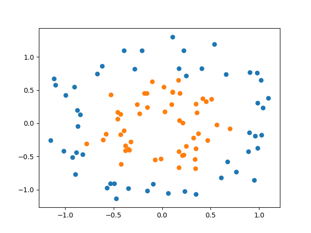
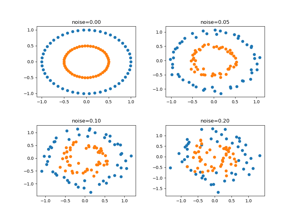
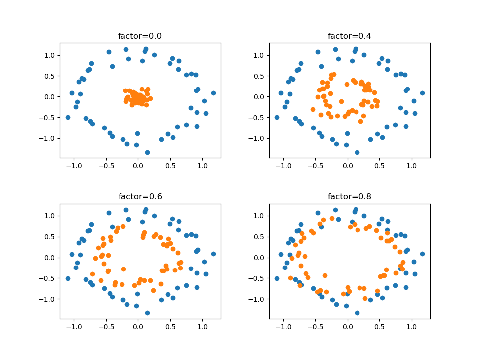
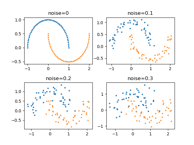
まずmake_circles()で2クラスのデータを生成し、外側のクラス0をblue、内側のクラス1をorangeとして再定義する。
|
1 2 3 4 5 6 7 |
import numpy as np from sklearn.ensemble import GradientBoostingClassifier from sklearn.datasets import make_circles from sklearn.model_selection import train_test_split X, y = make_circles(noise=0.25, factor=0.5, random_state=1) y_named = np.array(["blue", "orange"])[y] |
次に、データを訓練データとテストデータに分割し、訓練データによって学習する。データ分割にあたって、Xとyに加えて文字列に置き換えたy_namedを分割している。学習の際にはXとy_namedの訓練データとテストデータのみを用いるのでyについては特に含める必要ないが、ここではtrain_test_split()が3つ以上のデータでも分割可能なことを示している。
|
1 2 3 4 5 |
X_train, X_test, y_train, y_test, y_train_named, y_test_named = \ train_test_split(X, y, y_named, random_state=0) gbc = GradientBoostingClassifier(random_state=0) gbc.fit(X_train, y_train_named) |
学習後の分類器のclasses_プロパティーを参照すると、クラスがどのように表現されるかを確認できる。上のfit()メソッドでy_train_namedを与えたのでクラスの表現が文字列になっているが、代わりにy_trainを用いると[0, 1]のように元のyに対応したクラス表現が返される。
|
1 2 3 |
print(gbc.classes_) # ['blue' 'orange'] |
次に、学習済みモデルにテストデータを与えて、decision_function()の結果とpredict()の結果を並べてみる。decision_function()はfit()で与えたテストデータ数の1次元配列を返し、各要素の負の値に対してクラス0のblueが、正の値に対してはクラス1のorangeがpredict()で予測されていることがわかる。
|
1 2 3 4 5 6 7 8 9 10 11 12 13 14 15 16 17 18 19 20 21 22 23 24 25 26 27 28 29 30 31 |
data = DataFrame() data["decision_value"] = gbc.decision_function(X_test) data["prediction"] = gbc.predict(X_test) print(data) # decision_value prediction # 0 4.135926 orange # 1 -1.701699 blue # 2 -3.951061 blue # 3 -3.626096 blue # 4 4.289866 orange # 5 3.661661 orange # 6 -7.690972 blue # 7 4.110017 orange # 8 1.107539 orange # 9 3.407822 orange # 10 -6.462560 blue # 11 4.289866 orange # 12 3.901563 orange # 13 -1.200312 blue # 14 3.661661 orange # 15 -4.172312 blue # 16 -1.230101 blue # 17 -3.915762 blue # 18 4.036028 orange # 19 4.110017 orange # 20 4.110017 orange # 21 0.657090 orange # 22 2.698263 orange # 23 -2.656733 blue # 24 -1.867766 blue |
decision_function()の各要素の符号に応じてpredict()と同じ結果を得たいなら、次のように処理していくとよい。
|
1 2 3 4 5 6 7 8 9 10 11 12 |
print(gbc.decision_function(X_test) > 0) # [ True False False False True True False True True True False True # True False True False False False True True True True True False # False] print((gbc.decision_function(X_test) > 0).astype(int)) # [1 0 0 0 1 1 0 1 1 1 0 1 1 0 1 0 0 0 1 1 1 1 1 0 0] print(gbc.classes_[(gbc.decision_function(X_test) > 0).astype(int)]) # ['orange' 'blue' 'blue' 'blue' 'orange' 'orange' 'blue' 'orange' 'orange' # 'orange' 'blue' 'orange' 'orange' 'blue' 'orange' 'blue' 'blue' 'blue' # 'orange' 'orange' 'orange' 'orange' 'orange' 'blue' 'blue'] |
最後に、上記のデータと正解であるy_test_namedのデータを先ほどのデータフレームに追加して全体を確認する。predit()メソッドの結果とdecision_function()の符号による判定結果は等しく、y_testと異なるデータがあることがわかる。
|
1 2 3 4 5 6 7 8 9 10 11 12 13 14 15 16 17 18 19 20 21 22 23 24 25 26 27 28 29 30 31 32 |
data["decision"] = \ gbc.classes_[(gbc.decision_function(X_test) > 0).astype(int)] data["y_test"] = y_test_named print(data) # decision_value prediction decision y_test # 0 4.135926 orange orange orange # 1 -1.701699 blue blue blue # 2 -3.951061 blue blue blue # 3 -3.626096 blue blue blue # 4 4.289866 orange orange orange # 5 3.661661 orange orange orange # 6 -7.690972 blue blue blue # 7 4.110017 orange orange orange # 8 1.107539 orange orange orange # 9 3.407822 orange orange orange # 10 -6.462560 blue blue blue # 11 4.289866 orange orange orange # 12 3.901563 orange orange orange # 13 -1.200312 blue blue orange # 14 3.661661 orange orange orange # 15 -4.172312 blue blue orange # 16 -1.230101 blue blue orange # 17 -3.915762 blue blue blue # 18 4.036028 orange orange orange # 19 4.110017 orange orange orange # 20 4.110017 orange orange blue # 21 0.657090 orange orange orange # 22 2.698263 orange orange orange # 23 -2.656733 blue blue blue # 24 -1.867766 blue blue blue |
decision_function()の意味
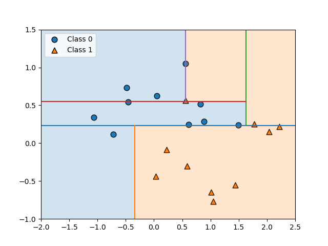
decusuib_function()のレベルは超平面上の高さになるが、これはデータ、モデルパラメーターにより変化し、このスケールの解釈は難しい。それはpredict_proba()で得られる予測確率とdecision_function()で計算される確信度の非線形性からも予想される。
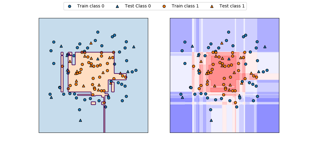
circlesデータに対するGradientBoostingClassifierの決定境界とdecision_function()の値の分布を表示したのが以下の図。コンターが交錯していてわかりにくく、直感的にはpredict_proba()の方がわかりやすい。
|
1 2 3 4 5 6 7 8 9 10 11 12 13 14 15 16 17 18 19 20 21 22 23 24 25 26 27 28 29 30 31 32 33 34 35 36 37 38 39 40 41 42 43 44 45 46 47 48 49 50 51 |
import numpy as np import matplotlib.pyplot as plt from sklearn.datasets import make_circles from sklearn.model_selection import train_test_split from sklearn.ensemble import GradientBoostingClassifier f0min, f0max = -1.5, 1.5 f1min, f1max = -1.75, 1.5 X, y = make_circles(noise=0.25, factor=0.5, random_state=1) X_train, X_test, y_train, y_test =\ train_test_split(X, y, random_state=0) gb = GradientBoostingClassifier(random_state=0) gb.fit(X_train, y_train) print("X_test.shape : {}".format(X_test.shape)) print("Decision function shape: {}".format( gb.decision_function(X_test).shape)) fig, axs = plt.subplots(1, 2, figsize=(10, 4.8)) color0, color1 = 'tab:blue', 'tab:orange' f0 = np.linspace(f0min, f0max, 200) f1 = np.linspace(f1min, f1max, 200) f0, f1 = np.meshgrid(f0, f1) F = np.c_[f0.reshape(-1, 1), f1.reshape(-1, 1)] pred = gb.predict(F).reshape(f0.shape) axs[0].contour(f0, f1, pred, levels=[0.5]) axs[0].contourf(f0, f1, pred, levels=1, colors=[color0, color1], alpha=0.25) decision = gb.decision_function(F).reshape(f0.shape) axs[1].contourf(f0, f1, decision, alpha=0.5, cmap='bwr') for ax in axs: ax.scatter(X_train[y_train==0][:, 0], X_train[y_train==0][:, 1], marker='o', fc=color0, ec='k', label="Train class 0") ax.scatter(X_test[y_test==0][:, 0], X_test[y_test==0][:, 1], marker='^', fc=color0, ec='k', label="Test Class 0") ax.scatter(X_train[y_train==1][:, 0], X_train[y_train==1][:, 1], marker='o', fc=color1, ec='k', label="Train class 1") ax.scatter(X_test[y_test==1][:, 0], X_test[y_test==1][:, 1], marker='^', fc=color1, ec='k', label="Test class 1") ax.set_xlim(f0min, f0max) ax.set_ylim(f1min, f1max) ax.tick_params(left=False, bottom=False, labelleft=False, labelbottom=False) handles, labels = axs[0].get_legend_handles_labels() fig.legend(handles, labels, ncol=4, loc='upper center') plt.show() |
3クラス以上の場合
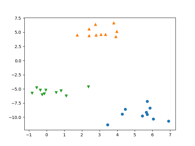
3クラスのirisデータセットにGradientBoostingClassifierを適用して、decision_function()の出力を見てみる。
|
1 2 3 4 5 6 7 8 9 10 11 12 13 14 15 16 17 18 19 20 21 |
import numpy as np from sklearn.datasets import load_iris from sklearn.model_selection import train_test_split from sklearn.ensemble import GradientBoostingClassifier from pandas import DataFrame iris = load_iris() X_train, X_test, y_train, y_test = train_test_split( iris.data, iris.target, random_state=42) gbc = GradientBoostingClassifier(learning_rate=0.01, random_state=0) gbc.fit(X_train, y_train) dec_func = gbc.decision_function(X_test) print(dec_func.shape) df = DataFrame(dec_func, columns=iris.target_names) df["decision"] = np.argmax(dec_func, axis=1) df["prediction"] = gbc.predict(X_test) print(df) |
このコードの出力結果は以下の通り。2クラスの場合は1次元配列だったが、3クラスになると行数×列数がデータ数×クラス数の配列になる。predict_proba()は2クラスでも2列の配列になるので、decision_function()の2クラスの場合だけ特に1次元配列になると言える。
なお、19行目で各データごとに最大の値をとる列をargmaxで探して、そのサフィックスを”decision”のクラス番号として表示している。
|
1 2 3 4 5 6 7 8 9 10 11 12 13 |
(38, 3) setosa versicolor virginica decision prediction 0 -1.995715 0.047583 -1.927207 1 1 1 0.061464 -1.907557 -1.927938 0 0 2 -1.990582 -1.876379 0.096867 2 2 3 -1.995715 0.047583 -1.927207 1 1 4 -1.997302 -0.134691 -1.203415 1 1 ..... 33 0.061464 -1.907557 -1.927938 0 0 34 0.061464 -1.907557 -1.927938 0 0 35 -1.997122 -1.876379 0.041660 2 2 36 -1.995715 0.047583 -1.927207 1 1 37 0.061464 -1.907557 -1.927938 0 0 |