準備
長方形の面積最大化
たとえば2変数の問題として、長方形の周囲長 を一定として、その面積が最大となる長方形の形状と面積はどのようになるかを考える。この場合、長方形の辺の長さを
 とすると、問題は以下のように表せる。
(1) 
これは以下のように代数的に簡単に解けて、答えは正方形とわかる。
(2) 
ただし変数の数が増えたり、目的関数や制約条件が複雑になると、解析的に解くのが面倒になる。
Lgrangeの未定乗数法による解
解法から先に示す。Lagrangeの未定乗数法では、目的関数 に対して以下の問題となる。
(3) 
 を最大化するために、
 で偏微分した以下の方程式を設定する。
(4) 
これを計算すると
(5) 
Lagrangeの未定乗数法の一般形
一般には、変数 について、目的関数
 を制約条件
を制約条件 の下で最大化/最小化する問題として与えられる。
(6) 
この等式制約条件付き最大化/最小化問題は、以下のように を導入して、連立方程式として表現される。
(7) 
例題
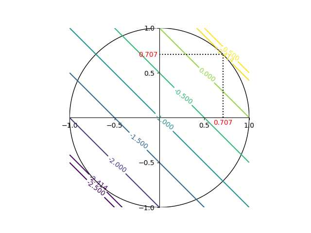
例題1:平面と円
平面 について、制約条件
 の下での極値を求める。
(8) 
lagrangeの未定乗数を導入して問題を定式化すると以下のようになる。
(9) 
(10) 
この連立方程式を解くと以下のようになり、解として2つの極値を得るが、それらは最大値と最小値に相当する。
(11) 
これを目的関数のコンターと制約条件の線で表すと以下の通り。
1 2 3 4 5 6 7 8 9 10 11 12 13 14 15 16 17 18 19 20 21 22 23 24 25 26 27 28 29 30 31 32 33 34 35 36 37 38 39 40 |
import numpy as np import matplotlib.pyplot as plt import matplotlib.patches as patches x = np.linspace(-1, 1, 20) y = np.linspace(-1, 1, 20) x, y = np.meshgrid(x, y) z = x + y - 1 fig = plt.figure() ax = fig.add_subplot(111) cntr = ax.contour(x, y, z ,levels=[-2.5, -2.414, -2, -1.5, -1, -0.5, 0, 0.414, 0.5]) ax.clabel(cntr) crc = patches.Circle(xy=(0, 0), radius=1, fill=False) ax.add_patch(crc) s2 = 1 / np.sqrt(2) ax.plot((0, s2), (s2, s2), c='k', linestyle='dotted') ax.plot((s2, s2), (0, s2), c='k', linestyle='dotted') ax.set_xlim((-1, 1)) ax.set_ylim((-1, 1)) ax.set_xticks([-1, -0.5, 0.5, 1]) ax.set_yticks([-1, -0.5, 0.5, 1]) ax.spines['bottom'].set_position('zero') ax.spines['left'].set_position('zero') ax.spines['right'].set_visible(False) ax.spines['top'].set_visible(False) ax.text(0.6, -0.08, "0.707", c='r') ax.text(-0.23, 0.68, "0.707", c='r') ax.set_aspect('equal') plt.show() |
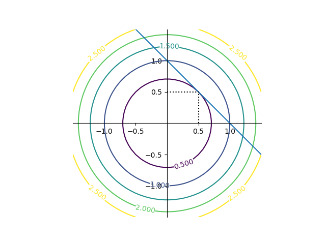
例題2:凸関数と直線
下に凸な関数について、直線 の制約条件下での最小値を求める。
(12) 
ここでlagrangeの未定乗数を導入して問題を定式化すると以下のようになる。
(13) 
(14) 
この連立方程式を解くと以下のようになり、解は最小値1つとなる。
(15) 
これを目的関数のコンターと制約条件の線で表すと以下の通り。
1 2 3 4 5 6 7 8 9 10 11 12 13 14 15 16 17 18 19 20 21 22 23 24 25 26 27 28 29 30 31 |
import numpy as np import matplotlib.pyplot as plt x = np.linspace(-1.5, 1.5, 40) y = np.linspace(-1.5, 1.5, 40) x, y = np.meshgrid(x, y) z = x * x + y * y fig = plt.figure() ax = fig.add_subplot(111) cntr = ax.contour(x, y, z, levels=[0.5, 1, 1.5, 2, 2.5]) ax.clabel(cntr) ax.plot([-0.5, 1.5], [1.5, -0.5]) ax.plot((0, .5), (.5, .5), c='k', linestyle='dotted') ax.plot((.5, .5), (0, .5), c='k', linestyle='dotted') ax.set_xticks([-1, -0.5, 0.5, 1]) ax.set_yticks([-1, -0.5, 0.5, 1]) ax.spines['bottom'].set_position('zero') ax.spines['left'].set_position('zero') ax.spines['right'].set_visible(False) ax.spines['top'].set_visible(False) ax.set_aspect('equal') plt.show() |
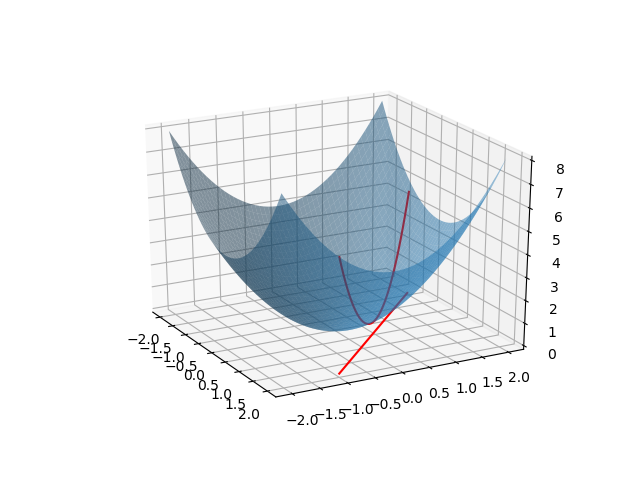
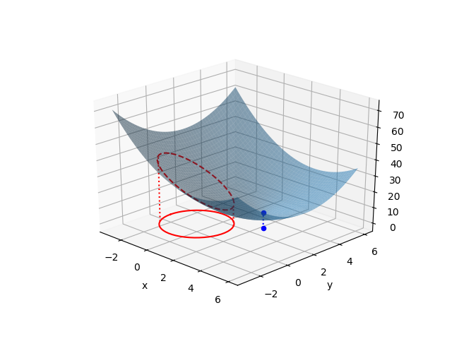
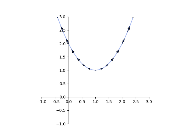
なお、これを3次元で表示すると以下のようになる。青い曲面が目的関数で、赤い直線が制約条件となる。最適化問題は、制約条件を満たす曲面上の点(図中、赤い放物線)の最小値を求めることになる。
1 2 3 4 5 6 7 8 9 10 11 12 13 14 15 16 17 18 19 20 21 22 23 24 25 26 27 28 29 |
import numpy as np import matplotlib.pyplot as plt from mpl_toolkits.mplot3d import Axes3D xmin, xmax = -2, 2 ymin, ymax = -2, 2 x = np.linspace(xmin, xmax) y = np.linspace(ymin, ymax) x_paraboloid, y_paraboloid = np.meshgrid(x, y) z_paraboloid = x_paraboloid**2 + y_paraboloid**2 x_constraint = x.copy() y_constraint = 1 - x z_constraint = x_constraint**2 + y_constraint**2 for i, v in enumerate(y_constraint): if v <= ymin or v >= ymax: x_constraint[i] = np.nan y_constraint[i] = np.nan z_constraint[i] = np.nan fig = plt.figure() ax = fig.add_subplot(111, projection='3d') ax.plot_surface(x_paraboloid, y_paraboloid, z_paraboloid, alpha=0.5) ax.plot(x_constraint, y_constraint, z_constraint, color='r') ax.plot(x_constraint, y_constraint, 0, color='r') plt.show() |
幾何学的説明
式(7)は以下のように書ける。
(16) ![\begin{gather*} \left[ \begin{array}{c} \dfrac{\partial f}{\partial x_1} \\ \vdots \\ \dfrac{\partial f}{\partial x_n} \end{array} \right] = \lambda \left[ \begin{array}{c} \dfrac{\partial g}{\partial x_1} \\ \vdots \\ \dfrac{\partial g}{\partial x_n} \end{array} \right] \\ g(x_1, \ldots, x_n) = 0 \end{gather*}](http://taustation.com/wp1/wp-content/ql-cache/quicklatex.com-c297beeeabd64856118393aad789fe1a_l3.png "Rendered by QuickLaTeX.com")
さらにgradientで表すと
(17) 
すなわちこの式の解 は、制約条件である
 を満足し、その曲線上にある。さらに解の点において
 の勾配ベクトルとゼロ平面上における
 の勾配ベクトルが平行になる。これはゼロ平面上の解の点において制約条件の曲線とのコンターのうち特定の曲線が接するのと同義であり、この点は停留点(stationary point)である。
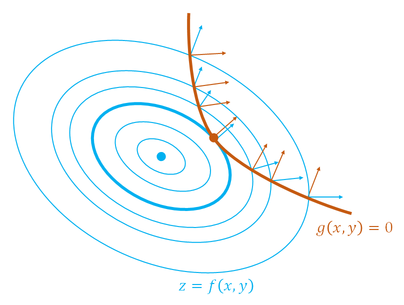
つまりこのような停留点を発見する手順は、制約条件を満たす(制約条件の線上にある)点のうち、その点において目的関数のgradientと制約条件の関数のgradientが平行となる点を求めるということになる。再度これを式で表すと、
(18) 
となるが、これをLangrange関数 と定義したうえで各変数で偏微分したものをゼロと置いた方程式を解くと表現している。未定乗数λは停留点における目的関数のgradientと制約条件の関数のgradientの比を表している。
λの符号
λの符号に意味があるかどうか。
たとえば、以下の制約条件付き最適化問題を考える。
(19) 
(20) 
この問題の制約条件を変更して以下のようにした場合。
(21) 
(22) 
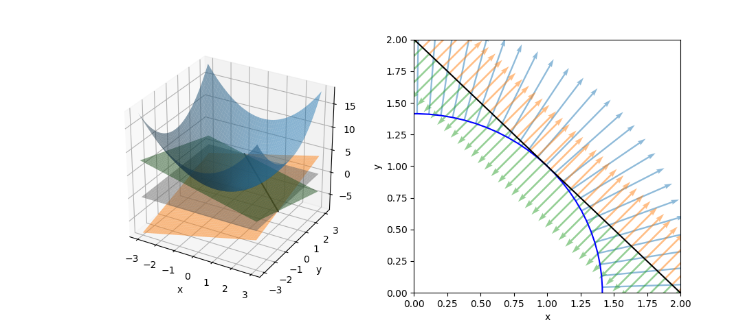
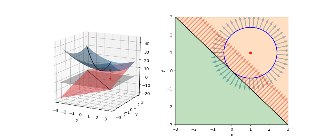
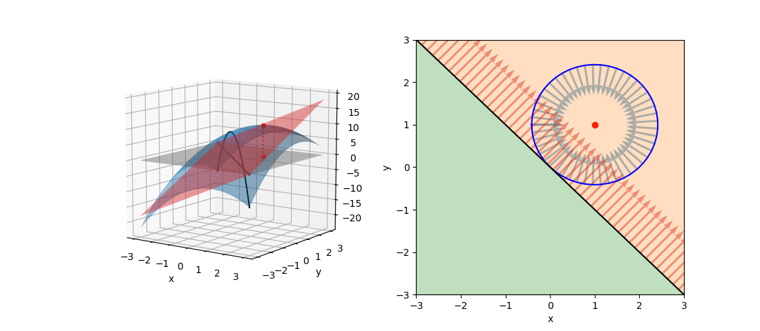
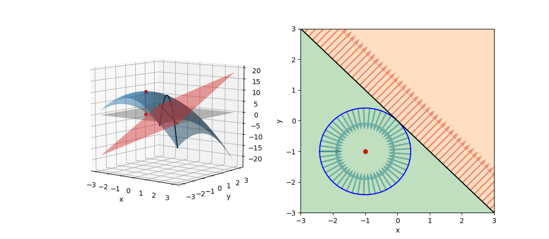
このように、制約条件の正負を反転するとλの符号が逆になるが解は変わらない。これを表したのが以下の図。
等式制約条件の場合、制約条件の線上でgradientが平行になりさえすればよいので、λ符号(制約条件式の正負)には拘らなくてよい。
1 2 3 4 5 6 7 8 9 10 11 12 13 14 15 16 17 18 19 20 21 22 23 24 25 26 27 28 29 30 31 32 33 34 35 36 37 38 39 40 41 42 43 44 45 46 47 48 49 50 51 52 53 54 55 56 57 |
import numpy as np import matplotlib.pyplot as plt import matplotlib.patches as patch from mpl_toolkits.mplot3d import Axes3D xmin, xmax = -3, 3 ymin, ymax = -3, 3 xls, xle = -1, 3 yls, yle = 3, -1 xs = np.linspace(xmin, xmax) ys = np.linspace(ymin, ymax) xm, ym = np.meshgrid(xs, ys) zero_plain = np.full_like(xm, 0) z_prb = xm**2 + ym**2 z_pl1 = xm + ym - 2 z_pl2 = - xm - ym + 2 r = np.sqrt(2) t = np.linspace(-np.pi, np.pi, num=100) xc = r * np.cos(t) yc = r * np.sin(t) uqc = 2 * xc vqc = 2 * yc xql = np.linspace(xls, xle, num=80) yql = np.linspace(yls, yle, num=80) uql1 = np.full_like(xql, 1) vql1 = np.full_like(yql, 1) uql2 = np.full_like(xql, -1) vql2 = np.full_like(yql, -1) fig = plt.figure(figsize=(11, 4.8)) ax1 = fig.add_subplot(121, projection='3d') ax2 = fig.add_subplot(122) ax1.plot_surface(xm, ym, zero_plain, color='gray', alpha=0.5) ax1.plot_surface(xm, ym, z_prb, color='tab:blue', alpha=0.5) ax1.plot_surface(xm, ym, z_pl1, color='tab:orange', alpha=0.5) ax1.plot_surface(xm, ym, z_pl2, color='tab:green', alpha=0.5) ax1.plot([xls, yls], [xle, yle], [0, 0], c='k') ax1.set_xlabel("x") ax1.set_ylabel("y") ax2.plot(xc, yc, c='b') ax2.plot([xls, yls], [xle, yle], c='k') ax2.quiver(xc, yc, uqc, vqc, scale_units='xy', scale=4, color='tab:blue', alpha=0.5) ax2.quiver(xql, yql, uql1, vql1, scale_units='xy', scale=4, color='tab:orange', alpha=0.5) ax2.quiver(xql, yql, uql2, vql2, scale_units='xy', scale=4, color='tab:green', alpha=0.5) ax2.set_xlabel("x") ax2.set_ylabel("y") ax2.set_xlim(0, 2) ax2.set_ylim(0, 2) plt.show() |
停留点が極致とならない例
以下の最適化問題の解をみてみる。
(23) 
(24) 
第1式から第2式を引き、第3式を適用して、
(25) 
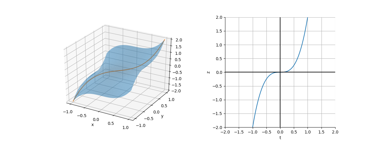
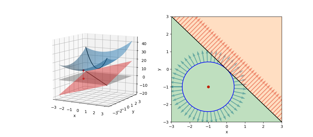
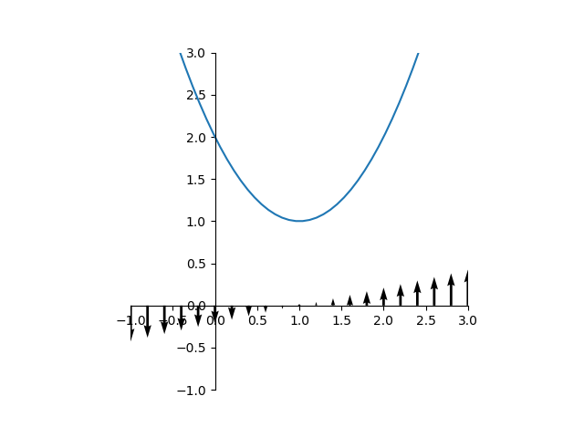
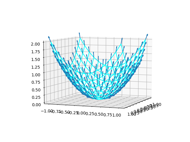
ここで の曲面と制約条件
 に対する曲面上の軌跡を描くと下図左のようになる。下図の右は
 として曲線を表したもので、
 で勾配は水平になっており、停留点ではあるが極大/極小となっていない。
1 2 3 4 5 6 7 8 9 10 11 12 13 14 15 16 17 18 19 20 21 22 23 24 25 26 27 28 29 30 31 32 33 34 35 36 37 |
import numpy as np import matplotlib.pyplot as plt from mpl_toolkits.mplot3d import Axes3D x = np.linspace(-1, 1) y = np.linspace(-1, 1) xs, ys = np.meshgrid(x, y) zs = xs**3 + ys**3 t = np.linspace(-1, 1) xp = yp = t zp = xp**3 + yp**3 fig = plt.figure(figsize=(13, 4.8)) ax1 = fig.add_subplot(121, projection='3d') ax2 = fig.add_subplot(122) ax1.plot_surface(xs, ys, zs, alpha=0.5) ax1.plot(xp, yp, zp) ax1.set_xlabel("x") ax1.set_ylabel("y") ax1.set_xticks(np.arange(-1, 1.5, 0.5)) ax1.set_yticks(np.arange(-1, 1.5, 0.5)) ax2.plot(t, zp) ax2.plot((-2, 2), (0, 0), c='k') ax2.plot((0, 0), (-2, 2), c='k') ax2.set_xlim(-2, 2) ax2.set_ylim(-2, 2) ax2.spines['top'].set_visible(False) ax2.spines['right'].set_visible(False) ax2.set_xlabel("t") ax2.set_ylabel("z") ax2.set_aspect('equal') ax2.grid(True) plt.show() |
参考サイト
本記事をまとめるにあたって、下記サイトが大変参考になったことに感謝したい。

![\begin{equation*} \boldsymbol{d} = \left[\begin{array}{c} u \\ v \end{array}\right] \quad , \quad \boldsymbol{h} = \left[\begin{array}{c} x_H - x_P \\ y_H - y_P \end{array}\right] \end{equation*}](http://taustation.com/wp1/wp-content/ql-cache/quicklatex.com-f2d871a718a0bf799c88fd4f3ffbf9ac_l3.png "Rendered by QuickLaTeX.com")


![\begin{align*} |\boldsymbol{h}|^2 &= (x_H - x_P)^2 + (y_H - y_P)^2 \\ &= \frac{ \begin{array}{l} \phantom{+}v^2(u^2+v^2)(x_0 - x_P)^2 \\ + u^2(u^2+v^2)(y_0 - y_P)^2 \\ - 2uv(u^2+v^2)(x_0 - x_P)(y_0 - y_P) \end{array} }{(u^2 + v^2)^2} \\ &= \frac{v^2(x_0 - x_P)^2 + u^2(y_0 - y_P)^2 - 2uv(x_0 - x_P)(y_0 - y_P)} {u^2 + v^2} \\ &= \frac{[v(x_0 - x_P) - u(y_0 - y_P)]^2}{u^2 + v^2} \\ &= \frac{(v x_0 - u y_0 - v x_P + v y_P)^2}{u^2 + v^2} \end{align*}](http://taustation.com/wp1/wp-content/ql-cache/quicklatex.com-0133d3c4f59238d65ef4986890dec581_l3.png "Rendered by QuickLaTeX.com")


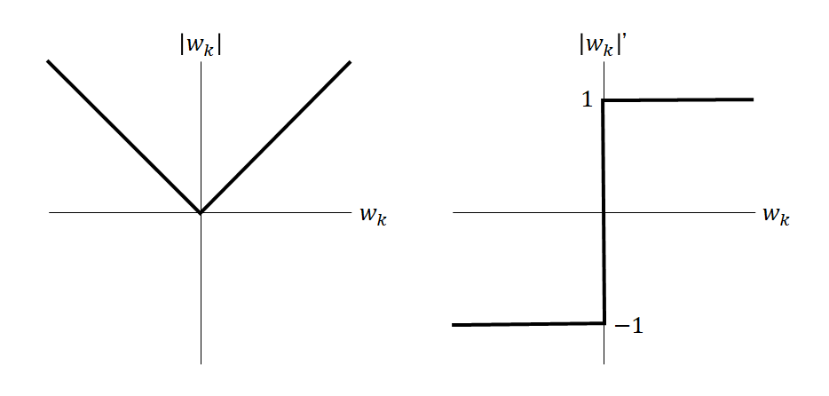
 と表し、左辺のwk以外に関わる項をMk、wkの係数となっている2乗和をSkkと表す。


![\begin{equation*} \frac{d |x|}{dx} = \left\{ \begin{array}{cl} -1 & (x < 0) \\ \left[ -1, 1 \right] & (x = 0) \\ 1 & (x > 0) \end{array} \right. \end{equation*}](http://taustation.com/wp1/wp-content/ql-cache/quicklatex.com-1aadd0e8e3a8da8daf0db2c69a068fd7_l3.png "Rendered by QuickLaTeX.com")
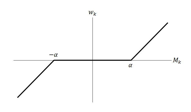
![\begin{gather*} w_k = 0 \quad \rightarrow \quad M_k +w_k S_{kk} + \alpha \left[ -1, 1 \right] = \left[ M_k - \alpha , M_k + \alpha \right] = 0\\ M_k - \alpha \le 0 \le M_k + \alpha \quad \rightarrow \quad -\alpha \le M_k \le \alpha \quad \rightarrow \quad w_k = 0 \end{gather*}](http://taustation.com/wp1/wp-content/ql-cache/quicklatex.com-567b5403ac4d6ca5907d235f1b760dcc_l3.png "Rendered by QuickLaTeX.com")


 と置いて最適化問題を解く。
 を満足する。この停留点が極値だということが分かっていれば、これが問題の解ということになる。
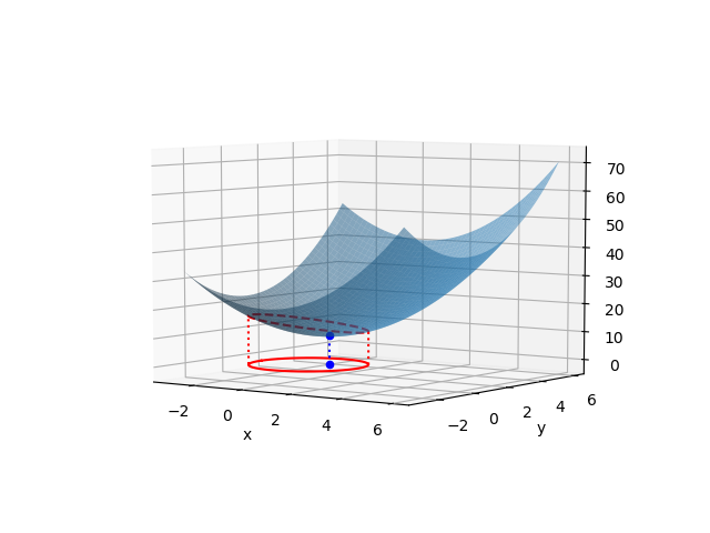

 として問題を解いてみる。
 の条件でLagrangeの未定乗数法によって解く。
 として、
として、


![\begin{equation*} \boldsymbol{x} = \left[ \begin{array}{c} x_1 \\ \vdots \\ x_n \\ \end{array} \right] \end{equation*}](http://taustation.com/wp1/wp-content/ql-cache/quicklatex.com-ca095fba05bd6b51953489329a4dbed5_l3.png "Rendered by QuickLaTeX.com")
![\begin{equation*} \boldsymbol{X} = \left[ \begin{array}{ccc} x_{11} & \ldots & x_{1n} \\ \vdots & x_{ij} & \vdots \\ x_{m1} & \ldots & x_{mn} \end{array} \right] \end{equation*}](http://taustation.com/wp1/wp-content/ql-cache/quicklatex.com-b789d485dcbf0314d7147eaf2ac533f1_l3.png "Rendered by QuickLaTeX.com")

![\begin{equation*} \boldsymbol{f}(x) = \left[ \begin{array}{c} f_1(x) \\ \vdots \\ f_n(x) \end{array} \right] \end{equation*}](http://taustation.com/wp1/wp-content/ql-cache/quicklatex.com-0c143adda5de76e2ad2d9f369b269daa_l3.png "Rendered by QuickLaTeX.com")
![\begin{equation*} \boldsymbol{f}(\boldsymbol{x}) =\ \left[ \begin{array}{c} f_1(x_1, \ldots, x_n) \\ \vdots \\ f_m(x_1, \ldots, x_n) \end{array} \right] \end{equation*}](http://taustation.com/wp1/wp-content/ql-cache/quicklatex.com-e1402f4bca526f4e708673a396a76432_l3.png "Rendered by QuickLaTeX.com")
![\begin{equation*} \boldsymbol{F}(x) = \left[ \begin{array}{ccc} F_{11}(x) & \ldots & F_{1n}(x) \\ \vdots & F_{ij} & \vdots \\ F_{m1}(x) & \ldots & F_{mn}(x) \\ \end{array} \right] \end{equation*}](http://taustation.com/wp1/wp-content/ql-cache/quicklatex.com-11b648294a10e1e0bd969847ac5eca32_l3.png "Rendered by QuickLaTeX.com")
![\begin{equation*} \frac{d \boldsymbol{f}(x)}{dx} = \left[ \begin{array}{c} \dfrac{d f_1(x)}{dx} \\ \vdots \\ \dfrac{d f_n(x)}{dx} \end{array} \right] \end{equation*}](http://taustation.com/wp1/wp-content/ql-cache/quicklatex.com-2a6538c824acdcefdc708eecff19c4c9_l3.png "Rendered by QuickLaTeX.com")
![\begin{equation*} \frac{d \boldsymbol{F}(x)}{dx} = \left[ \begin{array}{ccc} \dfrac{dF_{11}(x)}{dx} & \ldots & \dfrac{dF_{1n}(x)}{dx} \\ \vdots & \dfrac{dF_{ij}(x)}{dx} & \vdots \\ \dfrac{dF_{m1}(x)}{dx} & \ldots & \dfrac{dF_{mn}(x)}{dx} \end{array} \right] \end{equation*}](http://taustation.com/wp1/wp-content/ql-cache/quicklatex.com-fcd4c19cbe8c45de7a76c60b7e7414be_l3.png "Rendered by QuickLaTeX.com")
 のベクトルで微分すると、同じ次数のベクトルになる。
![\begin{equation*} \frac{df(\boldsymbol{x})}{d\boldsymbol{x}} = \left[ \begin{array}{c} \dfrac{\partial f}{\partial x_1} \\ \vdots \\ \dfrac{\partial f}{\partial x_m} \end{array} \right] \end{equation*}](http://taustation.com/wp1/wp-content/ql-cache/quicklatex.com-91df3f7d18edb4fce8d49b885fd8ba4d_l3.png "Rendered by QuickLaTeX.com")
![\begin{equation*} \frac{d}{d\boldsymbol{x}}f(\boldsymbol{x}) = \left[ \begin{array}{c} \dfrac{\partial}{\partial x_1} \\ \vdots \\ \dfrac{\partial}{\partial x_m} \end{array}\right] f(\boldsymbol{x}) \end{equation*}](http://taustation.com/wp1/wp-content/ql-cache/quicklatex.com-4f4019636c967a53d820033d665ac0e0_l3.png "Rendered by QuickLaTeX.com")
 の行列で微分すると、同じ次元・次数の行列になる。
![\begin{equation*} \frac{df(\boldsymbol{X})}{d\boldsymbol{X}} = \left[ \begin{array}{ccc} \dfrac{\partial f}{\partial x_{11}} & \ldots & \dfrac{\partial f}{\partial x_{1n}} \\ \vdots & \dfrac{\partial f}{\partial x_{ij}} & \vdots \\ \dfrac{\partial f}{\partial x_{m1}} & \ldots & \dfrac{\partial f}{\partial x_{mn}} \\ \end{array} \right] \end{equation*}](http://taustation.com/wp1/wp-content/ql-cache/quicklatex.com-420e553422141fba601f4663078d0386_l3.png "Rendered by QuickLaTeX.com")
![\begin{equation*} \frac{d}{d\boldsymbol{X}} f(\boldsymbol{X}) = \\ \left[ \begin{array}{ccc} \dfrac{\partial}{\partial x_{11}} & \ldots & \dfrac{\partial}{\partial x_{1n}} \\ \vdots & \dfrac{\partial}{\partial x_{ij}} & \vdots \\ \dfrac{\partial}{\partial x_{m1}} & \ldots & \dfrac{\partial}{\partial x_{mn}} \\ \end{array} \right] f(\boldsymbol{X}) \end{equation*}](http://taustation.com/wp1/wp-content/ql-cache/quicklatex.com-99d9e67383e94425fcf5d01ea0223e26_l3.png "Rendered by QuickLaTeX.com")
![\begin{equation*} \frac{d\boldsymbol{f}(\boldsymbol{x})^T}{d\boldsymbol{x}} = \left[ \begin{array}{ccc} \dfrac{\partial f_1}{\partial x_1} & \ldots & \dfrac{\partial f_n}{\partial x_1} \\ \vdots & \dfrac{\partial f_j}{\partial x_i} & \vdots \\ \dfrac{\partial f_1}{\partial x_m} & \ldots & \dfrac{\partial f_n}{\partial x_m} \\ \end{array} \right] \end{equation*}](http://taustation.com/wp1/wp-content/ql-cache/quicklatex.com-311d88dd2427ed7067a39ffafa8dad8d_l3.png "Rendered by QuickLaTeX.com")
![\begin{equation*} \frac{d}{d\boldsymbol{x}} \boldsymbol{f}(\boldsymbol{x})^T = \left[ \begin{array}{c} \dfrac{\partial}{\partial x_1} \\ \vdots \\ \dfrac{\parial}{\partial x_m} \end{array} \right] [ f_1(\boldsymbol{x}) \; \ldots \; f_n(\boldsymbol{x}) ] = \left[ \begin{array}{ccc} \dfrac{\partial f_1}{\partial x_1} & \cdots & \dfrac{\partial f_n}{\partial x_1} \\ & \dfrac{\partial f_j}{\partial x_i} &\\ \dfrac{\partial f_1}{\partial x_m} & \cdots & \dfrac{\partial f_n}{\partial x_m} \end{array} \right] \end{equation*}](http://taustation.com/wp1/wp-content/ql-cache/quicklatex.com-9a2aab5d164571bef0094ea7f1eaf975_l3.png "Rendered by QuickLaTeX.com")


![\begin{align*} \frac{df}{dx_i} &= \frac{\partial f}{\partial u_1}\frac{\partial u_1}{\partial x_i} + \cdots + \frac{\partial f}{\partial u_j}\frac{\partial u_j}{\partial x_i} + \cdots + \frac{\partial f}{\partial u_n}\frac{\partial u_n}{\partial x_i} \\ \rightarrow \frac{df(\boldsymbol{u}(\boldsymbol{x}))}{d\boldsymbol{x}} &= \left[ \begin{array}{ccc} \dfrac{\partial u_1}{\partial x_1} & \cdots & \dfrac{\partial u_n}{\partial x_1} \\ \vdots && \vdots \\ \dfrac{\partial u_1}{\partial x_m} & \cdots & \dfrac{\partial u_n}{\partial x_m} \\ \end{array} \right] \left[ \begin{array}{c} \dfrac{\partial f}{\partial u_1} \\ \vdots \\ \dfrac{\partial f}{\partial u_n} \end{array} \right] \\ &= \left[ \begin{array}{c} \dfrac{\partial}{\partial x_1} \\ \vdots \\ \dfrac{\partial}{\partial x_m} \end{array} \right] [u_1 \; \cdots \; u_n] \left[ \begin{array}{c} \dfrac{\partial}{\partial u_1} \\ \vdots \\ \dfrac{\partial}{\partial u_n} \end{array} \right] f(\boldsymbol{u}) \end{align*}](http://taustation.com/wp1/wp-content/ql-cache/quicklatex.com-299db8ffb5c52904ccea0f0f44844cb4_l3.png "Rendered by QuickLaTeX.com")

![\begin{align*} \frac{d(\boldsymbol{FG})}{dx} &= \frac{d}{dx}\left[\sum_{j=1}^m f_{ij} g_{jk}\right] = \left[\sum_{j=1}^m \left(\frac{df_{ij}}{dx} g_{jk} + f_{ij} \frac{dg_{jk}}{dx} \right)\right] \\ &= \left[ \sum_{j=1}^m \frac{df_{ij}}{dx} g_{jk} \right] + \left[ \sum_{j=1}^m f_{ij} \frac{dg_{jk}}{dx} \right] \end{align*}](http://taustation.com/wp1/wp-content/ql-cache/quicklatex.com-48367a30bf2176691b7825652e570751_l3.png "Rendered by QuickLaTeX.com")

![\begin{equation*} \begin{align} & \frac{d}{d\boldsymbol{x}} \left[ \begin{array}{c} a_{11}x_1 + \cdots + a_{1j}x_j + \cdots + a_{1n}x_n \\ \vdots \\ a_{i1}x_1 + \cdots + a_{ij}x_j + \cdots + a_{in}x_n \\ \vdots \\ a_{m1}x_1 + \cdots + a_{mj}x_j + \cdots + a_{mn}x_n \\ \end{array} \right]^T \\ &= \left[ \begin{array}{c} \dfrac{\partial}{\partial x_1} \\ \vdots \\ \dfrac{\partial}{\partial x_j} \\ \vdots \\ \dfrac{\partial}{\partial x_n} \\ \end{array} \right] \left[ \begin{array}{c} a_{11}x_1 + \cdots + a_{1j}x_j + \cdots + a_{1n}x_n \\ \vdots \\ a_{i1}x_1 + \cdots + a_{ij}x_j + \cdots + a_{in}x_n \\ \vdots \\ a_{m1}x_1 + \cdots + a_{mj}x_j + \cdots + a_{mn}x_n \\ \end{array} \right]^T \\ &= \left[ \begin{array}{ccccc} a_{11} & \cdots & a_{i1} & \cdots & a_{m1} \\ \vdots && \vdots && \vdots \\ a_{1j} & \cdots & a_{ij} & \cdots & a_{mj} \\ \vdots && \vdots && \vdots \\ a_{1n} & \cdots & a_{in} & \cdots & a_{mn} \\ \end{array} \right] = \boldsymbol{A}^T \end{align} \end{equation*}](http://taustation.com/wp1/wp-content/ql-cache/quicklatex.com-ae74fc9540924803afe8d58422df0a6f_l3.png "Rendered by QuickLaTeX.com")

![\begin{equation*} \left[ \begin{array}{c} \dfrac{\partial}{\partial x_1} \\ \vdots \\ \dfrac{\partial}{\partial x_n} \end{array} \right] [ x_1^2 + \cdots + x_n^2 ] = \left[ \begin{array}{c} 2x_1 \\ \vdots \\ 2x_n \end{array} \right] \end{equation*}](http://taustation.com/wp1/wp-content/ql-cache/quicklatex.com-9a4a53d35d99be2161876f0ebea4b973_l3.png "Rendered by QuickLaTeX.com")
 は正方行列で、
 と同じ次数でなければならない。
![\begin{align*} &\frac{d}{d \boldsymbol{x}} \left( [x_1 \; \cdots \; x_n] \left[ \begin{array}{ccc} a_{11} & \cdots & a_{1n} \\ \vdots & & \vdots \\ a_{n1} & \cdots & a_{nn} \\ \end{array} \right] \left[ \begin{array}{c} x_1 \\ \vdots \\ x_n \end{array} \right] \right)\\ &=\frac{d}{d \boldsymbol{x}} \left( [x_1 \; \cdots \; x_n] \left[ \begin{array}{c} a_{11} x_1 + \cdots + a_{1n} x_n \\ \vdots \\ a_{n1} x_1 + \cdots + a_{nn} x_n \end{array} \right] \right)\\ &= \frac{d}{d \boldsymbol{x}} \left( \left( a_{11} {x_1}^2 + \cdots + a_{1n} x_1 x_n \right) + \cdots + \left( a_{n1} x_n x_1 + \cdots + a_{nn} {x_n}^2 \right) \right) \end{array}\\ &=\left[ \begin{array}{c} \left( 2 a_{11} x_1 + \cdots + a_{1n} x_n \right) + a_{21} x_2 + \cdots + a_{n1} x_n \\ \vdots \\ a_{1n} x_1 + \cdots + a_{1n-1} x_{n-1} + \left( a_{n1} x_1 + \cdots + 2a_{nn} x_n \right) \end{array} \right] \\ &=\left[ \begin{array}{c} \left( a_{11} x_1 + \cdots + a_{1n} x_1 \right) + \left( a_{11} x_1 + \cdots + a_{n1} x_n \right) \\ \vdots \\ \left( a_{n1} x_1 + \cdots + a_{nn} x_n \right) + \left( a_{1n} x_1 + \cdots + a_{nn} x_n \right) \end{array} \right] \end{align*}](http://taustation.com/wp1/wp-content/ql-cache/quicklatex.com-deafe332adeef9ea5b9eb9c5cfbd1ef5_l3.png "Rendered by QuickLaTeX.com")


![\begin{align*} \left( [ \boldsymbol{AB} ]_{ij} \right)^T = \left( \sum_k \boldsymbol{A}_{ik} \boldsymbol{B}_{kj} \right)^T = \sum_k \boldsymbol{B}_{jk} \boldsymbol{A}_{ki} =\boldsymbol{B}^T \boldsymbol{A}^T \end{align*}](http://taustation.com/wp1/wp-content/ql-cache/quicklatex.com-e0a675c84ad11bc2c66bd764f6b3dfeb_l3.png "Rendered by QuickLaTeX.com")

![\begin{equation*} \left[ \begin{array}{ccc} a_{11} & \cdots & a_{1n} \\ \vdots & & \vdots \\ a_{m1} & \cdots & a_{mn} \\ \end{array} \right] \left[ \begin{array}{c} x_1 \\ \vdots \\ x_n \end{array} \right] = [x_1 \; \cdots \; x_n] \left[ \begin{array}{ccc} a_{11} & \cdots & a_{m1} \\ \vdots & & \vdots \\ a_{1n} & \cdots & a_{mn} \\ \end{array} \right] \end{equation*}](http://taustation.com/wp1/wp-content/ql-cache/quicklatex.com-47268abd1fb09618f4ac57dcd0edb815_l3.png "Rendered by QuickLaTeX.com")

![\begin{equation*} [x_1 \; \cdots \; x_n] \left[ \begin{array}{c} x_1 \\ \vdots \\ x_n \end{array} \right] = x_1^2 + \cdots + x_n^2 \end{equation*}](http://taustation.com/wp1/wp-content/ql-cache/quicklatex.com-d7eb4031678ac7ca0faa0eefd7cb4318_l3.png "Rendered by QuickLaTeX.com")


 は
は で極値を持ち、その前後で微分係数の符号が変わる。
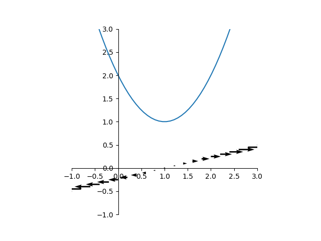
 を考えると、そのgradientは
 であり、ベクトル場は以下のようになる。
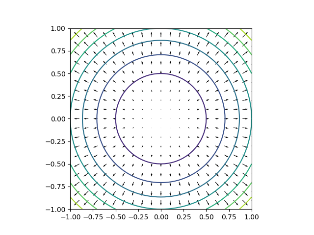
 方向で長さ1のベクトルを意味していて、これに対して


 、
、 とすると、
とすると、 の
の 方向の変化量の大きさは
 以下である。
 の
の


 の変化量が最も大きい。


 であり、上記の2次方程式の数は0個または1個である。

 、
、 とすると、ベクトルの内積となす角の関係から